API documentation
This page contains documentation which was automatically extracted from docstrings attached to the kafe2 source code. All major classes, methods and functions provided by kafe2 are documented here. For further information, or if in doubt about the exact functionality, users are invited to consult the source code itself. If you notice a mistake in the kafe2 documentation, or if you think that a particular part needs to be better documented, please open an issue on the kafe2 GitHub page.
kafe2 in a nutshell
Parameter estimation tools: fit
The kafe2.fit module provides an essential toolkit for estimating model
parameters from data (“fitting”).
It distinguishes between a number of different data types:
- series of indexed measurements (dedicated submodule:
indexed), - xy data (dedicated submodule:
xy), and - histograms (dedicated submodule:
histogram)
Each of the above data types has its own particularities when it comes to fitting. The main difference is due to the way uncertainties can be defined and interpreted for each type of data.
Indexed data
For indexed data, one data set consists of a list of  distinct measurements
 , with the (discrete) index
  ranging from
  to
to  .
For each measurement in the series, one or more uncertainty sources can be defined,
each being a numerical estimate of how much the respective measurement fluctuates.
Correlations between uncertainties on separate measurements and
.
For each measurement in the series, one or more uncertainty sources can be defined,
each being a numerical estimate of how much the respective measurement fluctuates.
Correlations between uncertainties on separate measurements and  can also
be taken into account by using covariance/correlation matrices.
can also
be taken into account by using covariance/correlation matrices.
Fits to indexed data take these uncertainties and correlations into account when estimating
the model parameters and their uncertainties. When plotting indexed data, measurements are
represented as data points with error bars at  , whereas the model
is indicated by a horizontal line near the corresponding data point.
, whereas the model
is indicated by a horizontal line near the corresponding data point.
The following objects are provided for handling indexed data, as described above:
IndexedContainer: data container for storing indexed dataIndexedParametricModel: corresponding model:- uses a model function (
IndexedModelFunction) to calculate the model predictions and stores the result in anIndexedContainer
- uses a model function (
IndexedFit: a fit of a parametric model to indexed data:- finds the minimum of the cost function to find the parameter values for which the model best fits the data
XY data
For xy data, the same principle as for indexed data applies, except each measurement and model prediction
now depends on a continuous real independent variable  instead of a discrete index .
In effect, the data now consist of ordered pairs
instead of a discrete index .
In effect, the data now consist of ordered pairs  .
.
In contrast to indexed data, where only uncertainties on the measurement could be defined,
for xy data there is the additional possibility of defining additional uncertainites on .
These can be handled in a number of different ways when fitting an xy model to data.
When plotting the result of xy fits, the model function is displayed as a continuous
function of , and an error band can be computed to reflect the model uncertainty,
as determined by propagating the data uncertainties.
The following objects are provided for handling xy data:
XYContainer: data container for storing xy dataXYParametricModel: corresponding model:- uses a model function (
XYModelFunction) to calculate the model predictions and stores the result in anXYContainer
- uses a model function (
XYFit: a fit of a parametric model to xy data:- finds the minimum of the cost function to find the parameter values for which the model best fits the data
Histograms
Finally, kafe2 is also able to handle histograms. Histograms organize measurements whose
values can fall anywhere across a continuum of values into a number of discrete regions
or “bins”. Typically, the continuous “measurement space” (a closed real interval ![[x_{\rm min}, x_{\rm max}]](../../_images/math/2a61990afcf5bac62f51bd7fb204bed6e6246097.png) )
is subdivided into a sequence of successive intervals at the “bin edges”
)
is subdivided into a sequence of successive intervals at the “bin edges”
 . Whenever a measurement falls into one of the bins, the
value of that histogram bin is incremented by one.
So a histogram is completely defined by its bin edges and the bin values.
. Whenever a measurement falls into one of the bins, the
value of that histogram bin is incremented by one.
So a histogram is completely defined by its bin edges and the bin values.
Note
The bin numbering starts at  for the first bin and ends at , where
is defined as the size of the histogram. The bin numbers and
for the first bin and ends at , where
is defined as the size of the histogram. The bin numbers and  refer to the
underflow (below
refer to the
underflow (below  ) and overflow bin (above
  ), respectively.
Defining a parametric model for histograms is not as straightforward as for xy and indexed data. Seeing as they keep track of the number of entries in different intervals of the continuum, the bin values can be interpreted using probability theory.
As the number of entries approaches infinity, the number of entries  in the bin covering an interval
 , divided by the total number of entries
  , will approach the probablity of an
event landing in that bin:
, will approach the probablity of an
event landing in that bin:
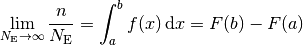
In the above formula,  is the probability distribution function (or probability density),
and
is the probability distribution function (or probability density),
and  is an antiderivative of
  (for example the cumulative probability distribution function).
Using the above relation, the model prediction  for the bin can be defined as:
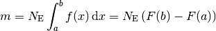
This means that, for histograms, the model density needs to be specified.
The model is then calculated by numerically integrating this function over each bin.
When fitting, however, the model needs to be calculated for many different points in parameter space,
which makes this approach very slow (many numerical integrations until the fit converges).
An alternative would be to specify the model density antiderviative  alongside
the model, so that the model can be calculated as a simple difference, rather than a complicated integral.
alongside
the model, so that the model can be calculated as a simple difference, rather than a complicated integral.
The following objects are provided for handling histograms:
HistContainer: data container for storing histogramsHistParametricModel: corresponding model:- uses a model function (
HistModelFunction) to calculate the model predictions and stores the result in anHistContainer
- uses a model function (
HistFit: a fit of a parametric model to histograms:- finds the minimum of the cost function to find the parameter values for which the model best fits the data
For creating graphical representations of fits, the Plot is provided. It can be instantiated
with any fit object (or list of fit objects) as an argument and will produce one or more plots accordingly
using matplotlib.
Tools for fitting series of indexed measurements (indexed)
-
class
kafe2.fit.indexed.IndexedContainer(data, dtype=<type 'float'>)¶ Bases:
kafe2.fit._base.container.DataContainerBaseThis object is a specialized data container for series of indexed measurements.
Construct a container for indexed data:
Parameters: - data (iterable of type <dtype>) – a one-dimensional array of measurements
- dtype (type) – data type of the measurements
-
size¶ number of data points
-
data¶ container data (one-dimensional
numpy.ndarray)
-
err¶ absolute total data uncertainties (one-dimensional
numpy.ndarray)
-
cov_mat¶ absolute data covariance matrix (
numpy.matrix)
-
cov_mat_inverse¶ inverse of absolute data covariance matrix (
numpy.matrix), orNoneif singular
-
cor_mat¶ absolute data correlation matrix (
numpy.matrix)
-
data_range¶ the minimum and maximum value of the data
Type: return
-
add_simple_error(err_val, name=None, correlation=0, relative=False)¶ Add a simple uncertainty source to the data container. Returns an error id which uniquely identifies the created error source.
Parameters: - err_val (float or iterable of float) – pointwise uncertainty/uncertainties for all data points
- name (str or
None) – unique name for this uncertainty source. IfNone, the name of the error source will be set to a random alphanumeric string. - correlation (float) – correlation coefficient between any two distinct data points
- relative (bool) – if
True, err_val will be interpreted as a relative uncertainty
Returns: error name
Return type: str
-
add_matrix_error(err_matrix, matrix_type, name=None, err_val=None, relative=False)¶ Add a matrix uncertainty source to the data container. Returns an error id which uniquely identifies the created error source.
Parameters: - err_matrix – covariance or correlation matrix
- matrix_type (str) – one of
'covariance'/'cov'or'correlation'/'cor' - name (str or
None) – unique name for this uncertainty source. IfNone, the name of the error source will be set to a random alphanumeric string. - err_val (iterable of float) – the pointwise uncertainties (mandatory if only a correlation matrix is given)
- relative (bool) – if
True, the covariance matrix and/or err_val will be interpreted as a relative uncertainty
Returns: error name
Return type: str
-
class
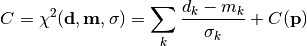
kafe2.fit.indexed.IndexedCostFunction_Chi2(errors_to_use='covariance', fallback_on_singular=True)¶ Bases:
kafe2.fit._base.cost.CostFunctionBase_Chi2Built-in least-squares cost function for histogram data.
Parameters: errors_to_use ( 'covariance','pointwise'orNone) – which erros to use when calculating
-
class
kafe2.fit.indexed.IndexedCostFunction_NegLogLikelihood(data_point_distribution='poisson')¶ Bases:
kafe2.fit._base.cost.CostFunctionBase_NegLogLikelihoodBuilt-in negative log-likelihood cost function for indexed data.
In addition to the measurement data and model predictions, likelihood-fits require a probability distribution describing how the measurements are distributed around the model predictions. This built-in cost function supports two such distributions: the Poisson and Gaussian (normal) distributions.
In general, a negative log-likelihood cost function is defined as the double negative logarithm of the product of the individual likelihoods of the data points.
Parameters: data_point_distribution ( 'poisson'or'gaussian') – which type of statistics to use for modelling the distribution of individual data points
-
class
kafe2.fit.indexed.IndexedCostFunction_NegLogLikelihoodRatio(data_point_distribution='poisson')¶ Bases:
kafe2.fit._base.cost.CostFunctionBase_NegLogLikelihoodRatioBuilt-in negative log-likelihood cost function for indexed data.
Warning
This cost function has not yet been properly tested and should not be used yet!
In addition to the measurement data and model predictions, likelihood-fits require a probability distribution describing how the measurements are distributed around the model predictions. This built-in cost function supports two such distributions: the Poisson and Gaussian (normal) distributions.
The likelihood ratio is defined as ratio of the likelihood function for each individual observation, divided by the so-called marginal likelihood.
Todo
Explain the above in detail.
Parameters: data_point_distribution ( 'poisson'or'gaussian') – which type of statistics to use for modelling the distribution of individual data points
-
class
kafe2.fit.indexed.IndexedCostFunction_UserDefined(user_defined_cost_function)¶ Bases:
kafe2.fit._base.cost.CostFunctionBaseUser-defined cost function for fits to series of indexed measurements. The function handle must be provided by the user.
Parameters: user_defined_cost_function – function handle Note
The names of the function arguments must be valid reserved names for the associated fit type (
IndexedFit)!
-
class
kafe2.fit.indexed.IndexedFit(data, model_function, cost_function=<kafe2.fit.indexed.cost.IndexedCostFunction_Chi2 object>, minimizer=None, minimizer_kwargs=None)¶ Bases:
kafe2.fit._base.fit.FitBaseConstruct a fit of a model to a series of indexed measurements.
Parameters: - data (iterable of float) – the measurement values
- model_function (
IndexedModelFunctionor unwrapped native Python function) – the model function - cost_function (
CostFunctionBase-derived or unwrapped native Python function) – the cost function - minimizer (None, "iminuit", "tminuit", or "scipy".) – the minimizer to use for fitting.
- minimizer_kwargs (dict) – dictionary with kwargs for the minimizer.
-
CONTAINER_TYPE¶ alias of
kafe2.fit.indexed.container.IndexedContainer
-
MODEL_TYPE¶ alias of
kafe2.fit.indexed.model.IndexedParametricModel
-
MODEL_FUNCTION_TYPE¶ alias of
kafe2.fit.indexed.model.IndexedModelFunction
-
PLOT_ADAPTER_TYPE¶ alias of
kafe2.fit.indexed.plot.IndexedPlotAdapter
-
EXCEPTION_TYPE¶ alias of
IndexedFitException
-
RESERVED_NODE_NAMES= set(['cost', 'data', 'data_cor_mat', 'data_cov_mat', 'data_error', 'model', 'model_cor_mat', 'model_cov_mat', 'model_error', 'total_cor_mat', 'total_cov_mat', 'total_error'])
-
data¶ array of measurement values
-
data_error¶ array of pointwise data uncertainties
-
data_cov_mat¶ the data covariance matrix
-
data_cov_mat_inverse¶ inverse of the data covariance matrix (or
Noneif singular)
-
data_cor_mat¶ the data correlation matrix
-
model¶ array of model predictions for the data points
-
model_error¶ array of pointwise model uncertainties
-
model_cov_mat¶ the model covariance matrix
-
model_cov_mat_inverse¶ inverse of the model covariance matrix (or
Noneif singular)
-
model_cor_mat¶ the model correlation matrix
-
total_error¶ array of pointwise total uncertainties
-
total_cov_mat¶ the total covariance matrix
-
total_cov_mat_inverse¶ inverse of the total covariance matrix (or
Noneif singular)
-
class
kafe2.fit.indexed.IndexedModelFunction(model_function)¶ Bases:
kafe2.fit._base.model.ModelFunctionBaseConstruct
IndexedModelFunctionobject (a wrapper for a native Python function):Parameters: model_function – function handle -
EXCEPTION_TYPE¶ alias of
IndexedModelFunctionException
-
FORMATTER_TYPE¶ alias of
kafe2.fit.indexed.format.IndexedModelFunctionFormatter
-
index_name¶ the name of the index variable
-
-
class
kafe2.fit.indexed.IndexedModelFunctionFormatter(name, latex_name=None, index_name='i', latex_index_name='i', arg_formatters=None, expression_string=None, latex_expression_string=None)¶ Bases:
kafe2.fit._base.format.ModelFunctionFormatterConstruct a
Formatterfor a model function for indexed data:Parameters: - name – a plain-text-formatted string indicating the function name
- latex_name – a LaTeX-formatted string indicating the function name
- index_name – a plain-text-formatted string representing the index
- latex_index_name – a LaTeX-formatted string representing the index
- arg_formatters – list of
ModelParameterFormatter-derived objects, formatters for function arguments - expression_string – a plain-text-formatted string indicating the function expression
- latex_expression_string – a LaTeX-formatted string indicating the function expression
-
get_formatted(with_par_values=True, n_significant_digits=2, format_as_latex=False, with_expression=False)¶ Get a formatted string representing this model function.
Parameters: - with_par_values – if
True, output will include the value of each function parameter (e.g.f_i(a=1, b=2, ...)) - n_significant_digits (int) – number of significant digits for rounding
- format_as_latex – if
True, the returned string will be formatted using LaTeX syntax - with_expression – if
True, the returned string will include the expression assigned to the function
Returns: string
- with_par_values – if
-
class
kafe2.fit.indexed.IndexedParametricModel(model_func, model_parameters, shape_like=None)¶ Bases:
kafe2.fit._base.model.ParametricModelBaseMixin,kafe2.fit.indexed.container.IndexedContainerConstruct an
IndexedParametricModelobject:Parameters: - model_func – handle of Python function (the model function)
- model_parameters – iterable of parameter values with which the model function should be initialized
- shape_like – array with the same shape as the model
-
data¶ model predictions (one-dimensional
numpy.ndarray)
-
data_range¶ tuple containing the minimum and maximum of all model predictions
-
eval_model_function(model_parameters=None)¶ Evaluate the model function.
Parameters: model_parameters (list or None) – values of the model parameters (ifNone, the current values are used)Returns: value(s) of the model function for the given parameters Return type: numpy.ndarray
-
eval_model_function_derivative_by_parameters(model_parameters=None, par_dx=None)¶ Evaluate the derivative of the model function with respect to the model parameters.
Parameters: - model_parameters (list or
None) – values of the model parameters (ifNone, the current values are used) - par_dx (float) – step size for numeric differentiation
Returns: value(s) of the model function derivative for the given parameters
Return type: numpy.ndarray- model_parameters (list or
-
class
kafe2.fit.indexed.IndexedPlotAdapter(indexed_fit_object)¶ Bases:
kafe2.fit._base.plot.PlotAdapterBaseConstruct an
IndexedPlotContainerfor aIndexedFitobject:Parameters: fit_object – an IndexedFitobject-
PLOT_STYLE_CONFIG_DATA_TYPE= 'indexed'
-
PLOT_SUBPLOT_TYPES= {'data': {'plot_adapter_method': 'plot_data', 'target_axes': 'main'}, 'model': {'plot_adapter_method': 'plot_model', 'target_axes': 'main'}, 'ratio': {'plot_adapter_method': 'plot_ratio', 'plot_style_as': 'data', 'target_axes': 'ratio'}}
-
data_x¶ data x values
-
data_y¶ data y values
-
data_xerr¶ NoneforIndexedPlotContainerType: x error bars for data
-
data_yerr¶ total data uncertainty
Type: y error bars for data
-
model_x¶ model prediction x values
-
model_y¶ model prediction y values
-
model_xerr¶ x error bars for model (actually used to represent the horizontal step length)
-
model_yerr¶ NoneforIndexedPlotContainerType: y error bars for model
-
x_range¶ (-0.5, N-0.5) for
IndexedPlotContainerType: x plot range
-
y_range¶ NoneforIndexedPlotContainerType: y plot range
-
plot_data(target_axes, **kwargs)¶ Plot the measurement data to a specified
matplotlibAxesobject.Parameters: - target_axes –
matplotlibAxesobject - kwargs – keyword arguments accepted by the
matplotlibmethodserrorbarorplot
Returns: plot handle(s)
- target_axes –
-
plot_model(target_axes, **kwargs)¶ Plot the model predictions to a specified matplotlib
Axesobject.Parameters: - target_axes –
matplotlibAxesobject - kwargs – keyword arguments accepted by the
step_fill_betweenmethod
Returns: plot handle(s)
- target_axes –
-
plot_ratio(target_axes, error_contributions=('data', ), **kwargs)¶ Plot the data/model ratio to a specified
matplotlibAxesobject.Parameters: - target_axes –
matplotlibAxesobject - kwargs – keyword arguments accepted by the
matplotlibmethodserrorbarorplot
Returns: plot handle(s)
- target_axes –
-
Tools for fitting xy data (xy)
-
class
kafe2.fit.xy.XYContainer(x_data, y_data, dtype=<type 'float'>)¶ Bases:
kafe2.fit.indexed.container.IndexedContainerThis object is a specialized data container for xy data.
Construct a container for xy data:
Parameters: - x_data (iterable of type <dtype>) – a one-dimensional array of measurement x values
- y_data (iterable of type <dtype>) – a one-dimensional array of measurement y values
- dtype (type) – data type of the measurements
-
size¶ number of data points
-
data¶ container data (both x and y, two-dimensional
numpy.ndarray)
-
x¶ container x data (one-dimensional
numpy.ndarray)
-
x_err¶ absolute total data x-uncertainties (one-dimensional
numpy.ndarray)
-
x_cov_mat¶ absolute data x covariance matrix (
numpy.matrix)
-
x_cov_mat_inverse¶ inverse of absolute data x covariance matrix (
numpy.matrix), orNoneif singular
-
x_cor_mat¶ absolute data x correlation matrix (
numpy.matrix)
-
y
-
y_err¶ absolute total data y-uncertainties (one-dimensional
numpy.ndarray)
-
y_cov_mat¶ absolute data y covariance matrix (
numpy.matrix)
-
y_cov_mat_inverse¶ inverse of absolute data y covariance matrix (
numpy.matrix), orNoneif singular
-
y_cor_mat¶ absolute data y correlation matrix (
numpy.matrix)
-
x_range¶ x data range
-
y_range¶ y data range
-
y_uncor_cov_mat
-
y_uncor_cov_mat_inverse
-
x_uncor_cov_mat
-
x_uncor_cov_mat_inverse
-
add_simple_error(axis, err_val, name=None, correlation=0, relative=False)¶ Add a simple uncertainty source for an axis to the data container. Returns an error id which uniquely identifies the created error source.
Parameters: - axis (str or int) –
'x'/0or'y'/1 - err_val (float or iterable of float) – pointwise uncertainty/uncertainties for all data points
- name (str or
None) – unique name for this uncertainty source. IfNone, the name of the error source will be set to a random alphanumeric string. - correlation (float) – correlation coefficient between any two distinct data points
- relative (bool) – if
True, err_val will be interpreted as a relative uncertainty
Returns: error id
Return type: int
- axis (str or int) –
-
add_matrix_error(axis, err_matrix, matrix_type, name=None, err_val=None, relative=False)¶ Add a matrix uncertainty source for an axis to the data container. Returns an error id which uniquely identifies the created error source.
Parameters: - axis (str or int) –
'x'/0or'y'/1 - err_matrix – covariance or correlation matrix
- matrix_type (str) – one of
'covariance'/'cov'or'correlation'/'cor' - name (str or
None) – unique name for this uncertainty source. IfNone, the name of the error source will be set to a random alphanumeric string. - err_val (iterable of float) – the pointwise uncertainties (mandatory if only a correlation matrix is given)
- relative (bool) – if
True, the covariance matrix and/or err_val will be interpreted as a relative uncertainty
Returns: error id
Return type: int
- axis (str or int) –
-
get_total_error(axis)¶ Get the error object representing the total uncertainty for an axis.
Parameters: axis (str or int) – 'x'/0or'y'/1Returns: error object representing the total uncertainty Return type: MatrixGaussianError
-
has_x_errors¶ Trueif at least one x uncertainty source is defined for the data container
-
has_uncor_x_errors¶ Trueif at least one x uncertainty source, which is not fully correlated, is defined for the data container
-
has_y_errors¶ Trueif at least one x uncertainty source is defined for the data container
-
class
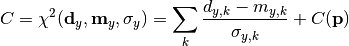
kafe2.fit.xy.XYCostFunction_Chi2(errors_to_use='covariance', fallback_on_singular=True, axes_to_use='xy')¶ Bases:
kafe2.fit._base.cost.CostFunctionBase_Chi2Built-in least-squares cost function for xy data.
Parameters: - errors_to_use (
'covariance','pointwise'orNone) – which errors to use when calculating - axes_to_use (
'y'or'xy') – take into account errors for which axes
-
on_no_errors()
-
static
chi2_no_errors(y_data, y_model, poi_values, parameter_constraints)¶ A least-squares cost function calculated from y data and model values, without considering uncertainties:

In the above,
 are the measurements,
 are the model predictions,
and
are the model predictions,
and  is the additional cost resulting from any constrained parameters.
Parameters: - y_data – y measurement data

- y_model – y model predictions

- poi_values – vector of parameters of interest

- parameter_constraints – list of fit parameter constraints
Returns: cost function value
- y_data – y measurement data
-
static
chi2_covariance(y_data, y_model, y_total_cov_mat_inverse, poi_values, parameter_constraints)¶ A least-squares cost function calculated from y data and model values, considering the covariance matrix of the y measurements.

In the above,
are the measurements,
are the model predictions,
 is the inverse of the total covariance matrix,
and is the additional cost resulting from any constrained parameters.
is the inverse of the total covariance matrix,
and is the additional cost resulting from any constrained parameters.Parameters: - y_data – y measurement data
- y_model – y model predictions
- y_total_cov_mat_inverse – inverse of the total covariance matrix

- poi_values – vector of parameters of interest
- parameter_constraints – list of fit parameter constraints
Returns: cost function value
- y_data – y measurement data
-
static
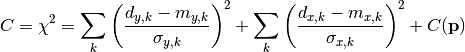
chi2_pointwise_errors(y_data, y_model, y_total_error, poi_values, parameter_constraints)¶ A least-squares cost function calculated from y data and model values, considering pointwise (uncorrelated) uncertainties for each data point:
In the above,
are the measurements,
are the model predictions,
 are the pointwise total uncertainties,
and is the additional cost resulting from any constrained parameters.
are the pointwise total uncertainties,
and is the additional cost resulting from any constrained parameters.Parameters: - y_data – y measurement data
- y_model – y model predictions
- y_total_error – total y error vector

- poi_values – vector of parameters of interest
- parameter_constraints – list of fit parameter constraints
Returns: cost function value
- y_data – y measurement data
-
static
chi2_xy_covariance(y_data, y_model, projected_xy_total_cov_mat_inverse, poi_values, parameter_constraints)
-
static
chi2_xy_pointwise_errors(y_data, y_model, projected_xy_total_error, poi_values, parameter_constraints)
-
static
chi2_pointwise_errors_fallback(y_data, y_model, y_total_error, poi_values, parameter_constraints)
-
static
chi2_covariance_fallback(y_data, y_model, y_total_cov_mat_inverse, poi_values, parameter_constraints)
-
static
chi2_xy_pointwise_errors_fallback(y_data, y_model, projected_xy_total_error, poi_values, parameter_constraints)
-
static
chi2_xy_covariance_fallback(y_data, y_model, projected_xy_total_cov_mat_inverse, poi_values, parameter_constraints)
- errors_to_use (
-
class
kafe2.fit.xy.XYCostFunction_Chi2_Nuisance(axes_to_use='xy', errors_to_use='covariance', fallback_on_singular=True)¶ Bases:
kafe2.fit._base.cost.CostFunctionBase_Chi2_NuisanceBuilt-in least-squares cost function with nuisanceparameters for xy data.
Parameters: - errors_to_use (
'covariance','pointwise'orNone) – which errors to use when calculating - axes_to_use (
'y'or'xy') – take into account errors for which axes
-
static
chi2_no_error(y_data, y_model, poi_values, parameter_constraints)¶ A least-squares cost function calculated from y data and model values, without considering uncertainties:

In the above,
are the measurements
are the model predictions,
are the model parameters,
and is the additional cost resulting from any constrained parameters.Parameters: - y_data – y measurement data
- y_model – y model predictions
- poi_values – vector of parameters of interest
- parameter_constraints – list of fit parameter constraints
Returns: cost function value
- y_data – y measurement data
-
static
chi2_nui_cov_y(y_data, y_model, y_total_uncor_cov_mat_inverse, _y_total_nuisance_cor_design_mat, y_nuisance_vector, poi_values, parameter_constraints)¶ A least-squares cost function which uses nuisance parameters to account for correlated y uncertainties.
The cost function is given by:

In the above,
are the y measurements,
are the y model predictions,
 is the design matrix containing the correlated parts of all y uncertainties,
 is the uncorrelated part of the total y covariance matrix,
 is the vector of nuisance parameters,
and is the additional cost resulting from any constrained parameters.
is the vector of nuisance parameters,
and is the additional cost resulting from any constrained parameters.Parameters: - y_data – y measurement data
- y_model – y model predictions
- y_total_uncor_cov_mat_inverse – inverse
 of the uncorrelated part of the total y covariance matrix
 - _y_total_nuisance_cor_design_mat – design matrix containing correlated y uncertainties
- y_nuisance_vector – nuisance parameter vector
- poi_values – vector of parameters of interest
- parameter_constraints – list of fit parameter constraints
Returns: cost function value
- y_data – y measurement data
-
static
chi2_nui_cov_fallback_y(y_data, y_model, y_total_uncor_cov_mat_inverse, _y_total_nuisance_cor_design_mat, y_nuisance_vector, poi_values, parameter_constraints)
-
static
chi2_nui_cov_x(y_data, y_model, x_total_uncor_cov_mat_inverse, x_model, x_data, poi_values, parameter_constraints)¶ A least-squares cost function which uses x nuisance parameters. The cost function is given by:

In the above,
are the y measurements,
are the y model predictions,
 are the x measurements,
 are the x model predictions,
 is the total uncorrelated x covariance matrix,
and is the additional cost resulting from any constrained parameters.
is the total uncorrelated x covariance matrix,
and is the additional cost resulting from any constrained parameters.Parameters: - y_data – y measurement data
- y_model – y model predictions
- x_data – x measurement data
- y_model – y model predictions
- x_total_uncor_cov_mat_inverse – inverse
 of the uncorrelated part of the total x covariance matrix
 - poi_values – vector of parameters of interest
- parameter_constraints – list of fit parameter constraints
Returns: cost function value
- y_data – y measurement data
-
static
chi2_nui_cov_fallback_x(y_data, y_model, x_total_uncor_cov_mat_inverse, x_model, x_data, poi_values, parameter_constraints)
-
static
chi2_nui_cov_xy(y_data, y_model, y_total_uncor_cov_mat_inverse, _y_total_nuisance_cor_design_mat, y_nuisance_vector, x_total_uncor_cov_mat_inverse, x_model, x_data, poi_values, parameter_constraints)¶ A least-squares cost function which uses x and y nuisance parameters The cost function is given by:

In the above,
are the y measurements, are the y model predictions,
are the x measurements, are the x model predictions,
is the design matrix containing the correlated parts of all y uncertainties,
is the total uncorrelated y covariance matrix,
is the total uncorrelated x covariance matrix,
and is the additional cost resulting from any constrained parameters.Parameters: - y_data – y measurement data
- y_model – y model predictions
- x_data – x measurement data
- x_model – x model predictions
- x_total_uncor_cov_mat_inverse – inverse of the uncorrelated part of the total x covariance matrix
- y_total_uncor_cov_mat_inverse – inverse of the uncorrelated part of the total y covariance matrix
- _y_total_nuisance_cor_design_mat – design matrix containing correlated y uncertainties
- poi_values – vector of parameters of interest
- y_nuisance_vector – nuisance parameter vector
Returns: cost function value
- y_data – y measurement data
-
static
chi2_nui_cov_fallback_xy(y_data, y_model, y_total_uncor_cov_mat_inverse, _y_total_nuisance_cor_design_mat, y_nuisance_vector, x_total_uncor_cov_mat_inverse, x_model, x_data, poi_values, parameter_constraints)
-
static
chi2_nui_pointwise_y(y_data, y_model, y_total_error, poi_values, parameter_constraints)¶ A least-squares cost function calculated from y data and model values, considering pointwise (uncorrelated) uncertainties for each data point:
In the above,
are the y measurements,
are the y model predictions,
are the pointwise total y uncertainties,
and is the additional cost resulting from any constrained parameters.Parameters: - y_data – y measurement data
- y_model – y model predictions
- y_total_error – total y error vector
- poi_values – vector of parameters of interest
- parameter_constraints – list of fit parameter constraints
Returns: cost function value
- y_data – y measurement data
-
static
chi2_nui_pointwise_fallback_y(y_data, y_model, y_total_error, poi_values, parameter_constraints)
-
static
chi2_nui_pointwise_x(y_data, y_model, x_total_error, x_model, x_data, poi_values, parameter_constraints)¶ A least-squares cost function taking pointwise x errors into account.
The cost function is given by:
In the above,
 are the y measurements,
  are the y model predictions,
 are the x measurements,
  are the x model predictions,
 are the total y errors,
 are the total x errors,
and is the additional cost resulting from any constrained parameters.
are the total x errors,
and is the additional cost resulting from any constrained parameters.Parameters: - y_data – y measurement data
- y_model – y model predictions
- x_data – x measurement data
- x_model – x model predictions
- x_total_error – total x error vector

- y_total_error – total y error vector
- poi_values – vector of parameters of interest
- parameter_constraints – list of fit parameter constraints
Returns: cost function value
- y_data – y measurement data
-
static
chi2_nui_pointwise_fallback_x(y_data, y_model, x_total_error, x_model, x_data, poi_values, parameter_constraints)
-
static
chi2_nui_pointwise_xy(y_data, y_model, x_total_error, x_model, x_data, y_total_error, poi_values, parameter_constraints)¶ A least-squares cost function taking pointwise x and y errors into account.
The cost function is given by:
In the above,
 are the y measurements,
  are the y model predictions,
are the x measurements,
are the y model predictions,
are the x measurements,  are the x model predictions,
are the total y errors,
are the total x errors,
and is the additional cost resulting from any constrained parameters.
are the x model predictions,
are the total y errors,
are the total x errors,
and is the additional cost resulting from any constrained parameters.Parameters: - y_data – y measurement data
- y_model – y model predictions
- x_data – x measurement data
- x_model – x model predictions
- x_total_error – total x error vector
- y_total_error – total y error vector
- poi_values – vector of parameters of interest
- parameter_constraints – list of fit parameter constraints
Returns: cost function value
- y_data – y measurement data
-
static
chi2_nui_pointwise_fallback_xy(y_data, y_model, x_total_error, x_model, x_data, y_total_error, poi_values, parameter_constraints)
- errors_to_use (
-
class
kafe2.fit.xy.XYCostFunction_NegLogLikelihood(data_point_distribution='poisson')¶ Bases:
kafe2.fit._base.cost.CostFunctionBase_NegLogLikelihoodBuilt-in negative log-likelihood cost function for xy data.
In addition to the measurement data and model predictions, likelihood-fits require a probability distribution describing how the measurements are distributed around the model predictions. This built-in cost function supports two such distributions: the Poisson and Gaussian (normal) distributions.
In general, a negative log-likelihood cost function is defined as the double negative logarithm of the product of the individual likelihoods of the data points.
Parameters: data_point_distribution ( 'poisson'or'gaussian') – which type of statistics to use for modelling the distribution of individual data points-
static
nll_gaussian(y_data, y_model, projected_xy_total_error, poi_values, parameter_constraints)¶ A negative log-likelihood function assuming Gaussian statistics for each measurement.
The cost function is given by:

In the above,
are the measurements,
are the model predictions,
are the pointwise total uncertainties,
and is the additional cost resulting from any constrained parameters.Parameters: - y_data – y measurement data
- y_model – y model predictions
- projected_xy_total_error – total xy error vector resulting from projecting x errors onto y errors
- poi_values – vector of parameters of interest
- parameter_constraints – list of fit parameter constraints
Returns: cost function value
- y_data – y measurement data
-
static
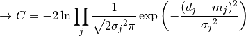
nll_poisson(y_data, y_model, poi_values, parameter_constraints)¶ A negative log-likelihood function assuming Poisson statistics for each measurement.
The cost function is given by:

In the above,
are the measurements,
are the model predictions,
and is the additional cost resulting from any constrained parameters.Parameters: - y_data – y measurement data
- y_model – y model predictions
- poi_values – vector of parameters of interest
- parameter_constraints – list of fit parameter constraints
Returns: cost function value
- y_data – y measurement data
-
static
-
class
kafe2.fit.xy.XYCostFunction_NegLogLikelihoodRatio(data_point_distribution='poisson')¶ Bases:
kafe2.fit._base.cost.CostFunctionBase_NegLogLikelihoodRatioBuilt-in negative log-likelihood cost function for xy data.
In addition to the measurement data and model predictions, likelihood-fits require a probability distribution describing how the measurements are distributed around the model predictions. This built-in cost function supports two such distributions: the Poisson and Gaussian (normal) distributions.
In general, a negative log-likelihood cost function is defined as the double negative logarithm of the product of the individual likelihoods of the data points.
Parameters: data_point_distribution ( 'poisson'or'gaussian') – which type of statistics to use for modelling the distribution of individual data points-
static
nllr_gaussian(y_data, y_model, projected_xy_total_error, poi_values, parameter_constraints)¶ A negative log-likelihood function assuming Gaussian statistics for each measurement.
The cost function is given by:
In the above,
are the measurements,
are the model predictions,
are the pointwise total uncertainties,
and is the additional cost resulting from any constrained parameters.Parameters: - y_data – y measurement data
- y_model – y model predictions
- projected_xy_total_error – total xy error vector resulting from projecting x errors onto y errors
- poi_values – vector of parameters of interest
- parameter_constraints – list of fit parameter constraints
Returns: cost function value
- y_data – y measurement data
-
static
nllr_poisson(y_data, y_model, poi_values, parameter_constraints)¶ A negative log-likelihood function assuming Poisson statistics for each measurement.
The cost function is given by:

In the above,
are the measurements,
are the model predictions,
and is the additional cost resulting from any constrained parameters.Parameters: - y_data – y measurement data
- y_model – y model predictions
- poi_values – vector of parameters of interest
- parameter_constraints – list of fit parameter constraints
Returns: cost function value
- y_data – y measurement data
-
static
-
class
kafe2.fit.xy.XYCostFunction_UserDefined(user_defined_cost_function)¶ Bases:
kafe2.fit._base.cost.CostFunctionBaseUser-defined cost function for fits to xy data. The function handle must be provided by the user.
Parameters: user_defined_cost_function – function handle Note
The names of the function arguments must be valid reserved names for the associated fit type (
XYFit)!
-
class
kafe2.fit.xy.XYFit(xy_data, model_function=<function linear_model>, cost_function=<kafe2.fit.xy.cost.XYCostFunction_Chi2 object>, x_error_algorithm='nonlinear', minimizer=None, minimizer_kwargs=None)¶ Bases:
kafe2.fit._base.fit.FitBaseConstruct a fit of a model to xy data.
Parameters: - xy_data ((2, N)-array of float) – the x and y measurement values
- model_function (
XYModelFunctionor unwrapped native Python function) – the model function - cost_function (
CostFunctionBase-derived or unwrapped native Python function) – the cost function - x_error_algorithm (str) – algorithm for handling x errors. Can be one of:
'iterative linear','nonlinear' - minimizer (None, "iminuit", "tminuit", or "scipy".) – the minimizer to use for fitting.
- minimizer_kwargs (dict) – dictionary with kwargs for the minimizer.
-
CONTAINER_TYPE¶ alias of
kafe2.fit.xy.container.XYContainer
-
MODEL_TYPE¶ alias of
kafe2.fit.xy.model.XYParametricModel
-
MODEL_FUNCTION_TYPE¶ alias of
kafe2.fit.xy.model.XYModelFunction
-
PLOT_ADAPTER_TYPE¶ alias of
kafe2.fit.xy.plot.XYPlotAdapter
-
EXCEPTION_TYPE¶ alias of
XYFitException
-
RESERVED_NODE_NAMES= set(['cost', 'nuisance_para', 'nuisance_y_data_cor_cov_mat', 'nuisance_y_model_cor_cov_mat', 'nuisance_y_total_cor_cov_mat', 'total_cor_mat', 'total_cor_mat_inversey_data_uncor_cov_mat', 'total_cov_mat', 'total_error', 'x_cor_mat', 'x_cov_mat', 'x_cov_mat_inverse', 'x_data_cov_mat', 'x_error', 'y_data', 'y_data_cor_mat', 'y_data_cov_mat', 'y_data_cov_mat_inverse', 'y_data_error', 'y_model', 'y_model_cor_mat', 'y_model_cov_mat', 'y_model_cov_mat_inverse', 'y_model_error', 'y_model_uncor_cov_mat', 'y_nuisance_vector', 'y_total_uncor_cov_mat'])
-
X_ERROR_ALGORITHMS= ('iterative linear', 'nonlinear')
-
has_x_errors¶ Trueif at least one x uncertainty source has been defined
-
has_y_errors¶ Trueif at least one y uncertainty source has been defined
-
x_data¶ array of measurement x values
-
x_label¶ x-label to be passed on to the plot
-
x_model
-
x_error¶ array of pointwise x uncertainties
-
x_cov_mat¶ the x covariance matrix
-
y_data¶ array of measurement data y values
-
y_label¶ y-label to be passed onto the plot
-
data¶ (2, N)-array containing x and y measurement values
-
model¶ (2, N)-array containing x and y model values
-
x_data_error¶ array of pointwise x data uncertainties
-
y_data_error¶ array of pointwise y data uncertainties
-
x_data_cov_mat¶ the data x covariance matrix
-
y_data_cov_mat¶ the data y covariance matrix
-
x_data_cov_mat_inverse¶ inverse of the data x covariance matrix (or
Noneif singular)
-
y_data_cov_mat_inverse¶ inverse of the data y covariance matrix (or
Noneif singular)
-
x_data_cor_mat¶ the data x correlation matrix
-
y_data_uncor_cov_mat¶ uncorrelated part of the data y covariance matrix (or
Noneif singular)
-
y_data_uncor_cov_mat_inverse¶ inverse of the uncorrelated part of the data y covariance matrix (or
Noneif singular)
-
x_data_uncor_cov_mat
-
x_data_uncor_cov_mat_inverse
-
y_data_cor_mat¶ the data y correlation matrix
-
y_model¶ array of y model predictions for the data points
-
x_model_error¶ array of pointwise model x uncertainties
-
y_model_error¶ array of pointwise model y uncertainties
-
x_model_cov_mat¶ the model x covariance matrix
-
y_model_cov_mat¶ the model y covariance matrix
-
x_model_cov_mat_inverse¶ inverse of the model x covariance matrix (or
Noneif singular)
-
y_model_cov_mat_inverse¶ inverse of the model y covariance matrix (or
Noneif singular)
-
y_model_uncor_cov_mat¶ uncorrelated part the model y covariance matrix
-
y_model_uncor_cov_mat_inverse¶ inverse of the uncorrelated part the model y covariance matrix (or
Noneif singular)
-
x_model_uncor_cov_mat¶ the model x uncorrelated covariance matrix
-
x_model_uncor_cov_mat_inverse¶ inverse of the model x uncorrelated covariance matrix (or
Noneif singular)
-
x_model_cor_mat¶ the model x correlation matrix
-
y_model_cor_mat¶ the model y correlation matrix
-
x_total_error¶ array of pointwise total x uncertainties
-
y_total_error¶ array of pointwise total y uncertainties
-
projected_xy_total_error¶ array of pointwise total y with the x uncertainties projected on top of them
-
x_total_cov_mat¶ the total x covariance matrix
-
y_total_cov_mat¶ the total y covariance matrix
-
projected_xy_total_cov_mat
-
x_total_cov_mat_inverse¶ inverse of the total x covariance matrix (or
Noneif singular)
-
y_total_cov_mat_inverse¶ inverse of the total y covariance matrix (or
Noneif singular)
-
projected_xy_total_cov_mat_inverse
-
y_total_uncor_cov_mat¶ the total y uncorrelated covariance matrix
-
y_total_uncor_cov_mat_inverse¶ inverse of the uncorrelated part of the total y covariance matrix (or
Noneif singular)
-
x_total_uncor_cov_mat¶ the total x uncorrelated covariance matrix
-
x_total_uncor_cov_mat_inverse¶ inverse of the total x uncorrelated covariance matrix (or
Noneif singular)
-
y_error_band¶ one-dimensional array representing the uncertainty band around the model function
-
x_range¶ range of the x measurement data
-
y_range¶ range of the y measurement data
-
poi_values
-
poi_names
-
x_uncor_nuisance_values¶ gives the x uncorrelated nuisance vector
-
add_simple_error(axis, err_val, name=None, correlation=0, relative=False, reference='data')¶ Add a simple uncertainty source for axis to the data container. Returns an error id which uniquely identifies the created error source.
Parameters: - axis (str or int) –
'x'/0or'y'/1 - err_val (float or iterable of float) – pointwise uncertainty/uncertainties for all data points
- correlation (float) – correlation coefficient between any two distinct data points
- relative (bool) – if
True, err_val will be interpreted as a relative uncertainty - reference ('data' or 'model') – which reference values to use when calculating absolute errors from relative errors
Returns: error id
Return type: int
- axis (str or int) –
-
add_matrix_error(axis, err_matrix, matrix_type, name=None, err_val=None, relative=False, reference='data')¶ Add a matrix uncertainty source for an axis to the data container. Returns an error id which uniquely identifies the created error source.
Parameters: - axis (str or int) –
'x'/0or'y'/1 - err_matrix – covariance or correlation matrix
- matrix_type (str) – one of
'covariance'/'cov'or'correlation'/'cor' - err_val (iterable of float) – the pointwise uncertainties (mandatory if only a correlation matrix is given)
- relative (bool) – if
True, the covariance matrix and/or err_val will be interpreted as a relative uncertainty - reference ('data' or 'model') – which reference values to use when calculating absolute errors from relative errors
Returns: error id
Return type: int
- axis (str or int) –
-
set_poi_values(param_values)¶ set the start values of all parameters of interests
-
do_fit()¶ Perform the fit.
-
eval_model_function(x=None, model_parameters=None)¶ Evaluate the model function.
Parameters: - x (iterable of float) – values of x at which to evaluate the model function (if
None, the data x values are used) - model_parameters (iterable of float) – the model parameter values (if
None, the current values are used)
Returns: model function values
Return type: numpy.ndarray- x (iterable of float) – values of x at which to evaluate the model function (if
-
calculate_nuisance_parameters()¶ Calculate and return the nuisance parameter values.
NOTE: currently only works for calculating nuisance parameters for correlated ‘y’ uncertainties.
Returns: vector containing the nuisance parameter values Return type: numpy.array
-
class
kafe2.fit.xy.XYFitEnsemble(n_experiments, x_support, model_function, model_parameters, cost_function=<kafe2.fit.xy.cost.XYCostFunction_Chi2 object>, requested_results=None)¶ Bases:
kafe2.fit._base.ensemble.FitEnsembleBaseObject for generating ensembles of fits to xy pseudo-data generated according to the specified uncertainty model.
After constructing an
XYFitEnsembleobject, an error model should be added to it. This is done as forXYFitobjects by using theadd_simple_errororadd_matrix_errormethods.Once an uncertainty model is provided, the fit ensemble can be generated by using the
runmethod. This method starts by generating a pseudo-dataset in such a way that the empirical distribution of the data corresponds to the specified uncertainty model. It then fits the model to the pseudo-data and extracts information from the fit, such as the resulting parameter values or the value of the cost function at the minimum. This is repeated a large number of times in order to evaluate the whole ensemble in a statistically meaningful way.The ensemble result can be visualized by using the
plot_resultsmethod.Construct an
XYFitEnsembleobject.Parameters: - n_experiments (int) – number of pseudoexperiments to perform
- x_support (iterable of float) – x values to use as support for calculating the “true” model (“true” x)
- model_function (
XYModelFunctionor unwrapped native Python function) – the model function - model_parameters (iterable of float) – parameters of the “true” model
- cost_function (
CostFunctionBase-derived or unwrapped native Python function) – the cost function - requested_results (iterable of str) – list of result variables to collect for each toy fit
-
FIT_TYPE¶ alias of
kafe2.fit.xy.fit.XYFit
-
AVAILABLE_STATISTICS= {'cor_mat': <property object>, 'cov_mat': <property object>, 'kurtosis': <property object>, 'mean': <property object>, 'mean_error': <property object>, 'skew': <property object>, 'std': <property object>}
-
n_exp¶ the number of pseudo-experiments to perform
-
n_par¶ the number of parameters
-
n_dat¶ the number of degrees of freedom for the fit
-
n_df¶ the number of degrees of freedom for the fit
-
add_simple_error(axis, err_val, name=None, correlation=0, relative=False, reference='data')¶ Add a simple uncertainty source for axis to the data container. Returns an error id which uniquely identifies the created error source.
Parameters: - axis (str or int) –
'x'/0or'y'/1 - err_val (float or iterable of float) – pointwise uncertainty/uncertainties for all data points
- correlation (float) – correlation coefficient between any two distinct data points
- relative (bool) – if
True, err_val will be interpreted as a relative uncertainty - reference ('data' or 'model') – which reference values to use when calculating absolute errors from relative errors
Returns: error id
Return type: int
- axis (str or int) –
-
add_matrix_error(axis, err_matrix, matrix_type, name=None, err_val=None, relative=False, reference='data')¶ Add a matrix uncertainty source for an axis to the data container. Returns an error id which uniquely identifies the created error source.
Parameters: - axis (str or int) –
'x'/0or'y'/1 - err_matrix – covariance or correlation matrix
- matrix_type (str) – one of
'covariance'/'cov'or'correlation'/'cor' - err_val (iterable of float) – the pointwise uncertainties (mandatory if only a correlation matrix is given)
- relative (bool) – if
True, the covariance matrix and/or err_val will be interpreted as a relative uncertainty - reference ('data' or 'model') – which reference values to use when calculating absolute errors from relative errors
Returns: error id
Return type: int
- axis (str or int) –
-
run()¶ Perform the pseudo-experiments. Retrieve and store the requested fit result variables.
-
get_results(*results)¶ Return a dictionary containing the ensembles of result variables.
Parameters: results (iterable of str. Calling without arguments retrieves all collected results.) – names of result variables to retrieve Returns: dict
-
get_results_statistics(results='all', statistics='all')¶ Return a dictionary containing statistics (e.g. mean) of the result variables.
Parameters: - results (iterable of str or
'all'(get statistics for all retrieved variables)) – names of retrieved fit variable for which to return statistics - statistics (iterable of str or
'all'(get all statistics for each retrieved variable)) – names of statistics to retrieve for each result variable
Returns: dict
- results (iterable of str or
-
plot_result_distributions(results='all', show_legend=True)¶ Make plots with histograms of the requested fit variable values across all pseudo-experiments.
Parameters: - results (iterable of str or
'all'(make plots for all retrieved variables)) – names of retrieved fit variable for which to generate plots - show_legend (bool) – if
True, show a plot legend on each figure
- results (iterable of str or
-
plot_result_scatter(results='all', show_legend=True)¶ Make plots with histograms of the requested fit variable values across all pseudo-experiments.
Parameters: - results (iterable of str or
'all'(make plots for all retrieved variables)) – names of retrieved fit variable for which to generate plots - show_legend (bool) – if
True, show a plot legend on each figure
- results (iterable of str or
-
AVAILABLE_RESULTS= {'cost': <property object>, 'parameter_pulls': <property object>, 'x_data': <property object>, 'y_data': <property object>, 'y_model': <property object>, 'y_pulls': <property object>}
-
class
kafe2.fit.xy.XYModelFunction(model_function=<function linear_model>)¶ Bases:
kafe2.fit._base.model.ModelFunctionBaseConstruct
XYModelFunctionobject (a wrapper for a native Python function):Parameters: model_function – function handle -
EXCEPTION_TYPE¶ alias of
XYModelFunctionException
-
FORMATTER_TYPE¶ alias of
kafe2.fit.xy.format.XYModelFunctionFormatter
-
x_name¶ the name of the independent variable
-
-
class
kafe2.fit.xy.XYModelFunctionFormatter(name, latex_name=None, x_name='x', latex_x_name=None, arg_formatters=None, expression_string=None, latex_expression_string=None)¶ Bases:
kafe2.fit._base.format.ModelFunctionFormatterConstruct a
Formatterfor a model function for xy data:Parameters: - name – a plain-text-formatted string indicating the function name
- latex_name – a LaTeX-formatted string indicating the function name
- x_name – a plain-text-formatted string representing the independent variable
- latex_x_name – a LaTeX-formatted string representing the independent variable
- arg_formatters – list of
ModelParameterFormatter-derived objects, formatters for function arguments - expression_string – a plain-text-formatted string indicating the function expression
- latex_expression_string – a LaTeX-formatted string indicating the function expression
-
get_formatted(with_par_values=True, n_significant_digits=2, format_as_latex=False, with_expression=False)¶ Get a formatted string representing this model function.
Parameters: - with_par_values – if
True, output will include the value of each function parameter (e.g.f_i(a=1, b=2, ...)) - n_significant_digits (int) – number of significant digits for rounding
- format_as_latex – if
True, the returned string will be formatted using LaTeX syntax - with_expression – if
True, the returned string will include the expression assigned to the function
Returns: string
- with_par_values – if
-
class
kafe2.fit.xy.XYParametricModel(x_data, model_func=<function linear_model>, model_parameters=[1.0, 1.0])¶ Bases:
kafe2.fit._base.model.ParametricModelBaseMixin,kafe2.fit.xy.container.XYContainerConstruct an
XYParametricModelobject:Parameters: - x_data – array containing the x values supporting the model
- model_func – handle of Python function (the model function)
- model_parameters – iterable of parameter values with which the model function should be initialized
-
data¶ model predictions (one-dimensional
numpy.ndarray)
-
x¶ model x support values
-
y¶ model y values
-
eval_model_function(x=None, model_parameters=None)¶ Evaluate the model function.
Parameters: - x (list or
None) – x values of the support points (ifNone, the model x values are used) - model_parameters (list or
None) – values of the model parameters (ifNone, the current values are used)
Returns: value(s) of the model function for the given parameters
Return type: numpy.ndarray- x (list or
-
eval_model_function_derivative_by_parameters(x=None, model_parameters=None, par_dx=None)¶ Evaluate the derivative of the model function with respect to the model parameters.
Parameters: - x (list or
None) – x values of the support points (ifNone, the model x values are used) - model_parameters (list or
None) – values of the model parameters (ifNone, the current values are used) - par_dx (float) – step size for numeric differentiation
Returns: value(s) of the model function derivative for the given parameters
Return type: numpy.ndarray- x (list or
-
eval_model_function_derivative_by_x(x=None, model_parameters=None, dx=None)¶ Evaluate the derivative of the model function with respect to the independent variable (x).
Parameters: - x (list or
None) – x values of the support points (ifNone, the model x values are used) - model_parameters (list or
None) – values of the model parameters (ifNone, the current values are used) - dx (float) – step size for numeric differentiation
Returns: value(s) of the model function derivative
Return type: numpy.ndarray- x (list or
-
class
kafe2.fit.xy.XYPlotAdapter(xy_fit_object, n_plot_points_model=100)¶ Bases:
kafe2.fit._base.plot.PlotAdapterBaseConstruct an
XYPlotContainerfor aXYFitobject:Parameters: fit_object – an XYFitobject-
PLOT_STYLE_CONFIG_DATA_TYPE= 'xy'
-
PLOT_SUBPLOT_TYPES= {'data': {'plot_adapter_method': 'plot_data', 'target_axes': 'main'}, 'model_error_band': {'plot_adapter_method': 'plot_model_error_band', 'target_axes': 'main'}, 'model_line': {'plot_adapter_method': 'plot_model_line', 'target_axes': 'main'}, 'ratio': {'plot_adapter_method': 'plot_ratio', 'plot_style_as': 'data', 'target_axes': 'ratio'}, 'ratio_error_band': {'plot_adapter_method': 'plot_ratio_error_band', 'plot_style_as': 'model_error_band', 'target_axes': 'ratio'}}
-
data_x¶ data x values
-
data_y¶ data y values
-
data_xerr¶ NoneforIndexedPlotContainerType: x error bars for data
-
data_yerr¶ total data uncertainty
Type: y error bars for data
-
model_x¶ model x values
-
model_y¶ model y values
-
model_xerr¶ NoneforIndexedPlotContainerType: x error bars for model
-
model_yerr¶ total model uncertainty
Type: y error bars for model
-
model_line_x¶ x support values for model function
-
model_line_y¶ y values at support points for model function
-
x_range¶ x plot range
-
y_range¶ NoneforXYPlotContainerType: y plot range
-
plot_data(target_axes, error_contributions=('data', ), **kwargs)¶ Plot the measurement data to a specified
matplotlibAxesobject.Parameters: - target_axes –
matplotlibAxesobject - kwargs – keyword arguments accepted by the
matplotlibmethodserrorbarorplot
Returns: plot handle(s)
- target_axes –
-
plot_model(target_axes, error_contributions=('model', ), **kwargs)¶ Plot the measurement data to a specified
matplotlibAxesobject.Parameters: - target_axes –
matplotlibAxesobject - kwargs – keyword arguments accepted by the
matplotlibmethodserrorbarorplot
Returns: plot handle(s)
- target_axes –
-
plot_model_line(target_axes, **kwargs)¶ Plot the model function to a specified matplotlib
Axesobject.Parameters: - target_axes –
matplotlibAxesobject - kwargs – keyword arguments accepted by the
matplotlibplotmethod
Returns: plot handle(s)
- target_axes –
-
plot_model_error_band(target_axes, **kwargs)¶ Plot an error band around the model model function.
Parameters: - target_axes –
matplotlibAxesobject - kwargs – keyword arguments accepted by the
matplotlibfill_betweenmethod
Returns: plot handle(s)
- target_axes –
-
plot_ratio(target_axes, error_contributions=('data', ), **kwargs)¶ Plot the data/model ratio to a specified
matplotlibAxesobject.Parameters: - target_axes –
matplotlibAxesobject - kwargs – keyword arguments accepted by the
matplotlibmethodserrorbarorplot
Returns: plot handle(s)
- target_axes –
-
plot_ratio_error_band(target_axes, **kwargs)¶ Plot model error band around the data/model ratio to a specified
matplotlibAxesobject.Parameters: - target_axes –
matplotlibAxesobject - kwargs – keyword arguments accepted by the
matplotlibmethodserrorbarorplot
Returns: plot handle(s)
- target_axes –
-
Tools for fitting histograms (histogram)
-
class
kafe2.fit.histogram.HistContainer(n_bins, bin_range, bin_edges=None, fill_data=None, dtype=<type 'int'>)¶ Bases:
kafe2.fit.indexed.container.IndexedContainerThis object is a specialized data container for organizing data into histograms.
A histogram is a compact representation of a potentially large number of entries which are distributed along a continuum of values. Histograms divide the continuum into intervals (“bins”) and count the number of entries per interval.
Construct a histogram:
Parameters: - n_bins (int) – number of bins
- bin_range (tuple of floats) – the lower and upper edges of the entire histogram
- bin_edges (list of floats) – the bin edges (if
None, each bin will have the same width) - fill_data (list of floats) – entries to fill into the histogram
- dtype (type) – data type of histogram entries
-
size¶ the number of bins (excluding underflow and overflow bins)
-
n_entries¶ the number of entries
-
data¶ the number of entries in each bin
-
raw_data¶ the number of entries in each bin
-
low¶ the lower edge of the histogram
-
high¶ the upper edge of the histogram
-
bin_range¶ a tuple containing the lower and upper edges of the histogram
-
overflow¶ the number of entries in the overflow bin
-
underflow¶ the number of entries in the underflow bin
-
n_bins¶ the number of bins
-
bin_edges¶ a list of the bin edges (including the outermost ones)
-
bin_widths¶ a list of the bin widths
-
bin_centers¶ a list of the (geometrical) bin centers
-
fill(entries)¶ Fill new entries into the histogram.
Parameters: entries (list of floats) – list of entries
-
rebin(new_bin_edges)¶ Change the histogram binning.
Parameters: new_bin_edges (list of float) – list of new bin edges in ascending order
-
class
kafe2.fit.histogram.HistCostFunction_Chi2(errors_to_use='covariance', fallback_on_singular=True)¶ Bases:
kafe2.fit._base.cost.CostFunctionBase_Chi2Built-in least-squares cost function for histogram data.
Parameters: errors_to_use ( 'covariance','pointwise'orNone) – which erros to use when calculating-
static
chi2_no_errors(data, model, parameter_values, parameter_constraints)¶ A least-squares cost function calculated from y data and model values, without considering uncertainties:
In the above,
are the measurements and are the model
predictions,
and is the additional cost resulting from any constrained parameters.Parameters: - data – measurement data
- model – model predictions
- parameter_values – vector of parameters
- parameter_constraints – list of fit parameter constraints
Returns: cost function value
- data – measurement data
-
static
chi2_covariance(data, model, total_cov_mat_inverse, parameter_values, parameter_constraints)¶ A least-squares cost function calculated from y data and model values, considering the covariance matrix of the y measurements.
In the above,
are the measurements, are the model
predictions, and is the inverse of the total covariance matrix,
and is the additional cost resulting from any constrained parameters.Parameters: - data – measurement data
- model – model predictions
- total_cov_mat_inverse – inverse of the total covariance matrix
- parameter_values – vector of parameters
- parameter_constraints – list of fit parameter constraints
Returns: cost function value
- data – measurement data
-
static
chi2_pointwise_errors(data, model, total_error, parameter_values, parameter_constraints)¶ A least-squares cost function calculated from y data and model values, considering pointwise (uncorrelated) uncertainties for each data point:
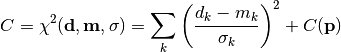
In the above,
are the measurements,
are the model predictions,
are the pointwise total uncertainties,
and is the additional cost resulting from any constrained parameters.Parameters: - data – measurement data
- model – model predictions
- total_error – total error vector
- parameter_values – vector of parameters
- parameter_constraints – list of fit parameter constraints
Returns: cost function value
- data – measurement data
-
static
-
class
kafe2.fit.histogram.HistCostFunction_NegLogLikelihood(data_point_distribution='poisson')¶ Bases:
kafe2.fit._base.cost.CostFunctionBase_NegLogLikelihoodBuilt-in negative log-likelihood cost function for Hist data.
In addition to the measurement data and model predictions, likelihood-fits require a probability distribution describing how the measurements are distributed around the model predictions. This built-in cost function supports two such distributions: the Poisson and Gaussian (normal) distributions.
In general, a negative log-likelihood cost function is defined as the double negative logarithm of the product of the individual likelihoods of the data points.
Parameters: data_point_distribution ( 'poisson'or'gaussian') – which type of statistics to use for modelling the distribution of individual data points-
static
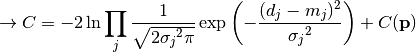
nll_gaussian(data, model, total_error, parameter_values, parameter_constraints)¶ A negative log-likelihood function assuming Gaussian statistics for each measurement.
The cost function is given by:
In the above,
are the measurements,
are the model predictions,
are the pointwise total uncertainties,
and is the additional cost resulting from any constrained parameters.Parameters: - data – measurement data
- model – model predictions
- total_error – total error vector
- parameter_values – vector of parameters
- parameter_constraints – list of fit parameter constraints
Returns: cost function value
- data – measurement data
-
static
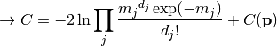
nll_poisson(data, model, parameter_values, parameter_constraints)¶ A negative log-likelihood function assuming Poisson statistics for each measurement.
The cost function is given by:
In the above,
are the measurements,
are the model predictions,
and is the additional cost resulting from any constrained parameters.Parameters: - data – measurement data
- model – model predictions
- parameter_values – vector of parameters
- parameter_constraints – list of fit parameter constraints
Returns: cost function value
- data – measurement data
-
static
-
class
kafe2.fit.histogram.HistCostFunction_NegLogLikelihoodRatio(data_point_distribution='poisson')¶ Bases:
kafe2.fit._base.cost.CostFunctionBase_NegLogLikelihoodRatioBuilt-in negative log-likelihood ratio cost function for histograms.
Warning
This cost function has not yet been properly tested and should not be used yet!
In addition to the measurement data and model predictions, likelihood-fits require a probability distribution describing how the measurements are distributed around the model predictions. This built-in cost function supports two such distributions: the Poisson and Gaussian (normal) distributions.
The likelihood ratio is defined as ratio of the likelihood function for each individual observation, divided by the so-called marginal likelihood.
Todo
Explain the above in detail.
Parameters: data_point_distribution ( 'poisson'or'gaussian') – which type of statistics to use for modelling the distribution of individual data points-
static
nllr_gaussian(data, model, total_error, parameter_values, parameter_constraints)¶ A negative log-likelihood function assuming Gaussian statistics for each measurement.
The cost function is given by:
In the above,
are the measurements,
are the model predictions,
are the pointwise total uncertainties,
and is the additional cost resulting from any constrained parameters.Parameters: - data – measurement data
- model – model predictions
- total_error – total y uncertainties for data
- parameter_values – vector of parameters
- parameter_constraints – list of fit parameter constraints
Returns: cost function value
- data – measurement data
-
static
nllr_poisson(data, model, parameter_values, parameter_constraints)¶ A negative log-likelihood function assuming Poisson statistics for each measurement.
The cost function is given by:
In the above,
are the measurements,
are the model predictions,
and is the additional cost resulting from any constrained parameters.Parameters: - data – measurement data
- model – model predictions
- parameter_values – vector of parameters
- parameter_constraints – list of fit parameter constraints
Returns: cost function value
- data – measurement data
-
static
-
class
kafe2.fit.histogram.HistCostFunction_UserDefined(user_defined_cost_function)¶ Bases:
kafe2.fit._base.cost.CostFunctionBaseUser-defined cost function for fits to histograms. The function handle must be provided by the user.
Parameters: user_defined_cost_function – function handle Note
The names of the function arguments must be valid reserved names for the associated fit type (
HistFit)!
-
class
kafe2.fit.histogram.HistFit(data, model_density_function=<function normal_distribution_pdf>, cost_function=<kafe2.fit.histogram.cost.HistCostFunction_NegLogLikelihood object>, model_density_antiderivative=None, minimizer=None, minimizer_kwargs=None)¶ Bases:
kafe2.fit._base.fit.FitBaseConstruct a fit of a model to a histogram.
Parameters: - data (
HistContainer) – aHistContainerrepresenting histogrammed data - model_density_function (
HistModelFunctionor unwrapped native Python function) – the model density function - cost_function (
CostFunctionBase-derived or unwrapped native Python function) – the cost function - minimizer (None, "iminuit", "tminuit", or "scipy".) – the minimizer to use for fitting.
- minimizer_kwargs (dict) – dictionary with kwargs for the minimizer.
-
CONTAINER_TYPE¶ alias of
kafe2.fit.histogram.container.HistContainer
-
MODEL_TYPE¶ alias of
kafe2.fit.histogram.model.HistParametricModel
-
MODEL_FUNCTION_TYPE¶ alias of
kafe2.fit.histogram.model.HistModelFunction
-
PLOT_ADAPTER_TYPE¶ alias of
kafe2.fit.histogram.plot.HistPlotAdapter
-
EXCEPTION_TYPE¶ alias of
HistFitException
-
RESERVED_NODE_NAMES= set(['cost', 'data', 'data_cor_mat', 'data_cov_mat', 'data_error', 'model', 'model_cor_mat', 'model_cov_mat', 'model_density', 'model_error', 'total_cor_mat', 'total_cov_mat', 'total_error'])
-
data¶ array of measurement values
-
data_error¶ array of pointwise data uncertainties
-
data_cov_mat¶ the data covariance matrix
-
data_cov_mat_inverse¶ inverse of the data covariance matrix (or
Noneif singular)
-
model¶ array of model predictions for the data points
-
model_error¶ array of pointwise model uncertainties
-
model_cov_mat¶ the model covariance matrix
-
model_cov_mat_inverse¶ inverse of the model covariance matrix (or
Noneif singular)
-
total_error¶ array of pointwise total uncertainties
-
total_cov_mat¶ the total covariance matrix
-
total_cov_mat_inverse¶ inverse of the total covariance matrix (or
Noneif singular)
-
eval_model_function_density(x, model_parameters=None)¶ Evaluate the model function density.
Parameters: - x (iterable of float) – values of x at which to evaluate the model function density
- model_parameters (iterable of float) – the model parameter values (if
None, the current values are used)
Returns: model function density values
Return type: numpy.ndarray
- data (
-
class
kafe2.fit.histogram.HistModelDensityFunctionFormatter(name, latex_name=None, x_name='x', latex_x_name=None, arg_formatters=None, expression_string=None, latex_expression_string=None)¶ Bases:
kafe2.fit._base.format.ModelFunctionFormatterConstruct a
Formatterfor a histogram model function density:Parameters: - name – a plain-text-formatted string indicating the function name
- latex_name – a LaTeX-formatted string indicating the function name
- x_name – a plain-text-formatted string representing the independent variable
- latex_x_name – a LaTeX-formatted string representing the independent variable
- arg_formatters – list of
ModelParameterFormatter-derived objects, formatters for function arguments - expression_string – a plain-text-formatted string indicating the function expression
- latex_expression_string – a LaTeX-formatted string indicating the function expression
-
get_formatted(with_par_values=True, n_significant_digits=2, format_as_latex=False, with_expression=False)¶ Get a formatted string representing this model function.
Parameters: - with_par_values – if
True, output will include the value of each function parameter (e.g.f_i(a=1, b=2, ...)) - n_significant_digits (int) – number of significant digits for rounding
- format_as_latex – if
True, the returned string will be formatted using LaTeX syntax - with_expression – if
True, the returned string will include the expression assigned to the function
Returns: string
- with_par_values – if
-
class
kafe2.fit.histogram.HistModelFunction(model_density_function=None, model_density_antiderivative=None)¶ Bases:
kafe2.fit._base.model.ModelFunctionBaseConstruct
XYModelFunctionobject (a wrapper for a native Python function):Parameters: - model_density_function – function handle
- model_density_antiderivative – function handle for model density antiderivative
-
EXCEPTION_TYPE¶ alias of
HistModelFunctionException
-
FORMATTER_TYPE¶ alias of
kafe2.fit.histogram.format.HistModelDensityFunctionFormatter
-
x_name¶ the name of the independent variable
-
antiderivative¶ model density antiderivative
-
class
kafe2.fit.histogram.HistParametricModel(n_bins, bin_range, model_density_func=<function normal_distribution_pdf>, model_parameters=[1.0, 1.0], bin_edges=None, model_density_func_antiderivative=None)¶ Bases:
kafe2.fit._base.model.ParametricModelBaseMixin,kafe2.fit.histogram.container.HistContainer-
data¶ model predictions (one-dimensional
numpy.ndarray)
-
eval_model_function_density(x, model_parameters=None)¶ Evaluate the model function density.
Parameters: - x (list of float) – x values of the support points
- model_parameters (list or
None) – values of the model parameters (ifNone, the current values are used)
Returns: value(s) of the model function for the given parameters
Return type: numpy.ndarray
-
fill(entries)¶ Fill new entries into the histogram.
Parameters: entries (list of floats) – list of entries
-
-
class
kafe2.fit.histogram.HistPlotAdapter(hist_fit_object, n_plot_points_model_density=100)¶ Bases:
kafe2.fit._base.plot.PlotAdapterBaseConstruct an
HistPlotContainerfor aHistFitobject:Parameters: - fit_object – an
HistFitobject - n_plot_points_model_density – number of plot points to use for plotting the model density
-
PLOT_STYLE_CONFIG_DATA_TYPE= 'histogram'
-
PLOT_SUBPLOT_TYPES= {'data': {'plot_adapter_method': 'plot_data', 'target_axes': 'main'}, 'model': {'plot_adapter_method': 'plot_model', 'target_axes': 'main'}, 'model_density': {'plot_adapter_method': 'plot_model_density', 'target_axes': 'main'}, 'ratio': {'plot_adapter_method': 'plot_ratio', 'plot_style_as': 'data', 'target_axes': 'ratio'}}
-
data_x¶ data x values
-
data_y¶ data y values
-
data_xerr¶ x error bars for data (actually used to represent the bins)
-
data_yerr¶ total data uncertainty
Type: y error bars for data
-
model_x¶ model prediction x values
-
model_y¶ model prediction y values
-
model_xerr¶ x error bars for model (actually used to represent the bins)
-
model_yerr¶ NoneforHistPlotContainerType: y error bars for model
-
model_density_x¶ x support points for model density plot
-
model_density_y¶ value of model density at the support points
-
x_range¶ x plot range (the histogram bin range)
-
y_range¶ NoneforIndexedPlotContainerType: y plot range
-
plot_data(target_axes, **kwargs)¶ Plot the measurement data to a specified
matplotlibAxesobject.Parameters: - target_axes –
matplotlibAxesobject - kwargs – keyword arguments accepted by the
matplotlibmethoderrorbar
Returns: plot handle(s)
- target_axes –
-
plot_model(target_axes, **kwargs)¶ Plot the model predictions to a specified matplotlib
Axesobject.Parameters: - target_axes –
matplotlibAxesobject - kwargs – keyword arguments accepted by the
matplotlibmethodbar
Returns: plot handle(s)
- target_axes –
-
plot_model_density(target_axes, **kwargs)¶ Plot the model density to a specified
matplotlibAxesobject.Parameters: - target_axes –
matplotlibAxesobject - kwargs – keyword arguments accepted by the
matplotlibmethodplot
Returns: plot handle(s)
- target_axes –
-
plot_ratio(target_axes, error_contributions=('data', ), **kwargs)¶ Plot the data/model ratio to a specified
matplotlibAxesobject.Parameters: - target_axes –
matplotlibAxesobject - kwargs – keyword arguments accepted by the
matplotlibmethodserrorbarorplot
Returns: plot handle(s)
- target_axes –
- fit_object – an
Abstract base classes (_base)
-
class
kafe2.fit._base.CostFunctionBase(cost_function)¶ Bases:
kafe2.fit.io.file.FileIOMixin,objectThis is a purely abstract class implementing the minimal interface required by all cost functions.
Any Python function returning a
floatcan be used as a cost function, although a number of common cost functions are provided as built-ins for all fit types.In order to be used as a model function, a native Python function must be wrapped by an object whose class derives from this base class. There is a dedicated
CostFunctionspecialization for each type of fit.This class provides the basic functionality used by all
CostFunctionobjects. These use introspection (inspect) for determining the parameter structure of the cost function and to ensure the function can be used as a cost function (validation).Construct
CostFunctionobject (a wrapper for a native Python function):Parameters: cost_function – function handle -
EXCEPTION_TYPE¶ alias of
CostFunctionException
-
FORMATTER_TYPE¶ alias of
kafe2.fit._base.format.CostFunctionFormatter
-
name¶ The cost function name (a valid Python identifier)
-
func¶ The cost function handle
-
signature¶ The model function argument specification, as returned by
inspect.signature
-
argcount¶ The number of arguments the model function accepts (including any independent variables which are not parameters)
-
argvals¶ The current values of the function arguments (not implemented, returns an array of zeros)
-
formatter¶ The
Formatterobject for this function
-
argument_formatters¶ The
Formatterobjects for the function arguments
-
ndf¶ The number of degrees of freedom of this cost function
-
needs_errors¶ Whether the cost function needs errors for a meaningful result
-
is_chi2¶ Whether the cost function is a chi2 cost function.
-
get_uncertainty_gaussian_approximation(data)¶ Get the gaussian approximation of the uncertainty inherent to the cost function, returns 0 by default. :param data: the fit data :return: the approximated gaussian uncertainty given the fit data
-
set_flag(name, value)
-
get_flag(name)
-
is_data_compatible(data)¶ Tests if model data is compatible with cost function :param data: the fit data :type data: numpy.ndarray :return: if the data is compatible, and if not a reason for the incompatibility :rtype: (boo, str)
-
on_no_errors()
-
-
class
kafe2.fit._base.CostFunctionBase_Chi2(errors_to_use='covariance', fallback_on_singular=True)¶ Bases:
kafe2.fit._base.cost.CostFunctionBaseBase class for built-in least-squares cost function.
Parameters: - errors_to_use (
'covariance','pointwise'orNone) – which errors to use when calculating - fallback_on_singular (bool) – if
Trueand the covariance matrix is singular (or the errors are zero), calculate as with errors_to_use=None
-
on_no_errors()
-
static
chi2_no_errors(data, model, parameter_values, parameter_constraints)¶ A least-squares cost function calculated from y data and model values, without considering uncertainties:
In the above,
are the measurements,
are the model predictions,
and is the additional cost resulting from any constrained parameters.Parameters: - data – measurement data
- model – model predictions
- parameter_values – vector of parameters
- parameter_constraints – list of fit parameter constraints
Returns: cost function value
- data – measurement data
-
static
chi2_covariance(data, model, total_cov_mat_inverse, parameter_values, parameter_constraints)¶ A least-squares cost function calculated from y data and model values, considering the covariance matrix of the y measurements.
In the above,
are the measurements,
are the model predictions,
is the inverse of the total covariance matrix,
and is the additional cost resulting from any constrained parameters.Parameters: - data – measurement data
- model – model predictions
- total_cov_mat_inverse – inverse of the total covariance matrix
- parameter_values – vector of parameters
- parameter_constraints – list of fit parameter constraints
Returns: cost function value
- data – measurement data
-
static
chi2_pointwise_errors(data, model, total_error, parameter_values, parameter_constraints)¶ A least-squares cost function calculated from y data and model values, considering pointwise (uncorrelated) uncertainties for each data point:
In the above,
are the measurements,
are the model predictions,
are the pointwise total uncertainties,
and is the additional cost resulting from any constrained parameters.Parameters: - data – measurement data
- model – model predictions
- total_error – total error vector
- parameter_values – vector of parameters
- parameter_constraints – list of fit parameter constraints
Returns: cost function value
- data – measurement data
-
static
chi2_covariance_fallback(data, model, total_cov_mat_inverse, parameter_values, parameter_constraints)
-
static
chi2_pointwise_errors_fallback(data, model, total_error, parameter_values, parameter_constraints)
- errors_to_use (
-
class
kafe2.fit._base.CostFunctionBase_NegLogLikelihood(data_point_distribution='poisson')¶ Bases:
kafe2.fit._base.cost.CostFunctionBaseBase class for built-in negative log-likelihood cost function.
In addition to the measurement data and model predictions, likelihood-fits require a probability distribution describing how the measurements are distributed around the model predictions. This built-in cost function supports two such distributions: the Poisson and Gaussian (normal) distributions.
In general, a negative log-likelihood cost function is defined as the double negative logarithm of the product of the individual likelihoods of the data points.
Parameters: data_point_distribution ( 'poisson'or'gaussian') – which type of statistics to use for modelling the distribution of individual data points-
static
nll_gaussian(data, model, total_error, parameter_values, parameter_constraints)¶ A negative log-likelihood function assuming Gaussian statistics for each measurement.
The cost function is given by:
In the above,
are the measurements,
are the model predictions,
are the pointwise total uncertainties,
and is the additional cost resulting from any constrained parameters.Parameters: - data – measurement data
- model – model predictions
- total_error – total error vector
- parameter_values – vector of parameters
- parameter_constraints – list of fit parameter constraints
Returns: cost function value
- data – measurement data
-
static
nll_poisson(data, model, parameter_values, parameter_constraints)¶ A negative log-likelihood function assuming Poisson statistics for each measurement.
The cost function is given by:
In the above,
are the measurements,
are the model predictions,
and is the additional cost resulting from any constrained parameters.Parameters: - data – measurement data
- model – model predictions
- parameter_values – vector of parameters
- parameter_constraints – list of fit parameter constraints
Returns: cost function value
- data – measurement data
-
is_data_compatible(data)¶ Tests if model data is compatible with cost function :param data: the fit data :type data: numpy.ndarray :return: if the data is compatible, and if not a reason for the incompatibility :rtype: (boo, str)
-
get_uncertainty_gaussian_approximation(data)¶ Get the gaussian approximation of the uncertainty inherent to the cost function, returns 0 by default. :param data: the fit data :return: the approximated gaussian uncertainty given the fit data
-
static
-
class
kafe2.fit._base.CostFunctionBase_NegLogLikelihoodRatio(data_point_distribution='poisson')¶ Bases:
kafe2.fit._base.cost.CostFunctionBaseBase class for built-in negative log-likelihood ratio cost function.
Warning
This cost function has not yet been properly tested and should not be used yet!
In addition to the measurement data and model predictions, likelihood-fits require a probability distribution describing how the measurements are distributed around the model predictions. This built-in cost function supports two such distributions: the Poisson and Gaussian (normal) distributions.
The likelihood ratio is defined as ratio of the likelihood function for each individual observation, divided by the so-called marginal likelihood.
Todo
Explain the above in detail.
Parameters: data_point_distribution ( 'poisson'or'gaussian') – which type of statistics to use for modelling the distribution of individual data points-
static
nllr_gaussian(data, model, total_error, parameter_values, parameter_constraints)¶ A negative log-likelihood ratio function assuming Gaussian statistics for each measurement.
The cost function is given by:
In the above,
are the measurements,
are the model predictions,
are the pointwise total uncertainties,
and is the additional cost resulting from any constrained parameters.Parameters: - data – measurement data
- model – model predictions
- total_error – total error vector
- parameter_values – vector of parameters
- parameter_constraints – list of fit parameter constraints
Returns: cost function value
- data – measurement data
-
static
nllr_poisson(data, model, parameter_values, parameter_constraints)¶ A negative log-likelihood function assuming Poisson statistics for each measurement.
The cost function is given by:
In the above,
are the measurements,
are the model predictions,
and is the additional cost resulting from any constrained parameters.Parameters: - data – measurement data
- model – model predictions
- parameter_values – vector of parameters
- parameter_constraints – list of fit parameter constraints
Returns: cost function value
- data – measurement data
-
is_data_compatible(data)¶ Tests if model data is compatible with cost function :param data: the fit data :type data: numpy.ndarray :return: if the data is compatible, and if not a reason for the incompatibility :rtype: (boo, str)
-
get_uncertainty_gaussian_approximation(data)¶ Get the gaussian approximation of the uncertainty inherent to the cost function, returns 0 by default. :param data: the fit data :return: the approximated gaussian uncertainty given the fit data
-
static
-
exception
kafe2.fit._base.CostFunctionException¶ Bases:
exceptions.Exception
-
class
kafe2.fit._base.CostFunctionFormatter(name, latex_name=None, arg_formatters=None, expression_string=None, latex_expression_string=None)¶ Bases:
kafe2.fit._base.format.ModelFunctionFormatterConstruct a
Formatterfor a model function:Parameters: - name – a plain-text-formatted string indicating the function name
- latex_name – a LaTeX-formatted string indicating the function name
- arg_formatters – list of
ModelParameterFormatter-derived objects, formatters for function arguments - expression_string – a plain-text-formatted string indicating the function expression
- latex_expression_string – a LaTeX-formatted string indicating the function expression
-
get_formatted(value=None, n_degrees_of_freedom=None, with_name=True, with_value_per_ndf=True, format_as_latex=False)¶ Get a formatted string representing this cost function.
Parameters: - value (float) – value of the cost function (if not
None, the returned string will include this) - n_degrees_of_freedom (int) – number of degrees of freedom (if not
None, the returned string will include this) - with_name – if
True, the returned string will include the cost function name - with_value_per_ndf – if
True, the returned string will include the value-ndf ratio as a decimal value - format_as_latex – if
True, the returned string will be formatted using LaTeX syntax
Returns: string
- value (float) – value of the cost function (if not
-
class
kafe2.fit._base.DataContainerBase¶ Bases:
kafe2.fit.io.file.FileIOMixin,objectThis is a purely abstract class implementing the minimal interface required by all types of data containers.
It stores measurement data and uncertainties.
-
size¶ The size of the data (number of measurement points)
-
data¶ A numpy array containing the data values
-
err¶ A numpy array containing the pointwise data uncertainties
-
cov_mat¶ A numpy matrix containing the covariance matrix of the data
-
cov_mat_inverse¶ A numpy matrix containing inverse of the data covariance matrix (or
Noneif not invertible)
-
has_errors¶ Trueif at least one uncertainty source is defined for the data container
-
add_simple_error(err_val, name=None, correlation=0, relative=False, reference=None)¶ Add a simple uncertainty source to the data container. Returns an error id which uniquely identifies the created error source.
Parameters: - err_val (float or iterable of float) – pointwise uncertainty/uncertainties for all data points
- name (str or
None) – unique name for this uncertainty source. IfNone, the name of the error source will be set to a random alphanumeric string. - correlation (float) – correlation coefficient between any two distinct data points
- relative (bool) – if
True, err_val will be interpreted as a relative uncertainty - reference (iterable of float or
None) – the data values to use when computing absolute errors from relative ones (and vice-versa)
Returns: error name
Return type: str
-
add_matrix_error(err_matrix, matrix_type, name=None, err_val=None, relative=False, reference=None)¶ Add a matrix uncertainty source to the data container. Returns an error id which uniquely identifies the created error source.
Parameters: - err_matrix – covariance or correlation matrix
- matrix_type (str) – one of
'covariance'/'cov'or'correlation'/'cor' - name (str or
None) – unique name for this uncertainty source. IfNone, the name of the error source will be set to a random alphanumeric string. - err_val (iterable of float) – the pointwise uncertainties (mandatory if only a correlation matrix is given)
- relative (bool) – if
True, the covariance matrix and/or err_val will be interpreted as a relative uncertainty - reference (iterable of float or
None) – the data values to use when computing absolute errors from relative ones (and vice-versa)
Returns: error name
Return type: str
-
disable_error(error_name)¶ Temporarily disable an uncertainty source so that it doesn’t count towards calculating the total uncertainty.
Parameters: error_name (str) – error name
-
enable_error(error_name)¶ (Re-)Enable an uncertainty source so that it counts towards calculating the total uncertainty.
Parameters: error_name (str) – error name
-
get_matching_errors(matching_criteria=None, matching_type='equal')¶ Return a list of uncertainty objects fulfilling the specified matching criteria.
Valid keys for
matching_criteria:name(the unique error name)type(eithersimpleormatrix)correlated(bool, only matches simple errors!)
NOTE: The error objects contained in the dictionary are not copies, but the original error objects. Modifying them is possible, but not recommended. If you do modify any of them, the changes will not be reflected in the total error calculation until the error cache is cleared. This can be done by calling the private method
_clear_total_error_cache.Parameters: - matching_criteria (dict or
None) – key-value pairs specifying matching criteria. The resulting error array will only contain error objects matching all provided criteria. IfNone, all error objects are returned. - matching_type (
'equal'or'regex') – how to perform the matching. If'equal', the value inmatching_criteriais checked for equality against the stored value. If'regex', the value in ``matching_criteriais interpreted as a regular expression and is matched against the stored value.
Returns: list of error objects
Return type: dict mapping error name to ~kafe2.core.error.GausianErrorBase-derived
-
get_error(error_name)¶ Return the uncertainty object holding the uncertainty.
NOTE: If you modify this object, the changes will not be reflected in the total error calculation until the error cache is cleared. This can be forced by calling
enable_error.Parameters: error_name (str) – error name Returns: error object Return type: ~kafe2.core.error.GausianErrorBase-derived
-
get_total_error()¶ Get the error object representing the total uncertainty.
Returns: error object representing the total uncertainty Return type: MatrixGaussianError
-
-
exception
kafe2.fit._base.DataContainerException¶ Bases:
exceptions.Exception
-
class
kafe2.fit._base.FitBase¶ Bases:
kafe2.fit.io.file.FileIOMixin,objectThis is a purely abstract class implementing the minimal interface required by all types of fitters.
-
CONTAINER_TYPE= None
-
MODEL_TYPE= None
-
PLOT_ADAPTER_TYPE= None
-
EXCEPTION_TYPE¶ alias of
FitException
-
RESERVED_NODE_NAMES= None
-
data
-
model
-
parameter_values¶ the current parameter values
-
parameter_names¶ the current parameter names
-
parameter_errors¶ the current parameter uncertainties
-
parameter_cov_mat¶ the current parameter covariance matrix
-
parameter_cor_mat¶ the current parameter correlation matrix
-
asymmetric_parameter_errors¶ the current asymmetric parameter uncertainties
-
parameter_name_value_dict¶ a dictionary mapping each parameter name to its current value
-
parameter_constraints¶ the gaussian constraints given for the fit parameters
-
cost_function_value¶ the current value of the cost function
-
data_size¶ the size (number of points) of the data container
-
has_model_errors¶ Trueif at least one uncertainty source is defined for the model
-
has_data_errors¶ Trueif at least one uncertainty source is defined for the data
-
has_errors¶ Trueif at least one uncertainty source is defined for either the data or the model
-
model_count¶ the number of model functions contained in the fit, 1 by default
-
poi_values¶ the values of the parameters of interest, equal to
self.parameter_valuesminus nuisance parameters
-
poi_names¶ the names of the parameters of interest, equal to
self.parameter_namesminus nuisance parameter names
-
did_fit¶ whether a fit was performed for the given data and model
-
ndf
-
set_parameter_values(**param_name_value_dict)¶ Set the fit parameters to new values. Valid keyword arguments are the names of the declared fit parameters.
Parameters: param_name_value_dict – new parameter values
-
set_all_parameter_values(param_value_list)¶ Set all the fit parameters at the same time.
Parameters: param_value_list – list of parameter values (mind the order)
-
fix_parameter(name, value=None)¶ Fix a parameter so that its value doesn’t change when calling
self.do_fit.Parameters: - name (str) – The name of the parameter to be fixed
- value (float) – The value to be given to the fixed parameter, optional
-
release_parameter(par_name)¶ Release a fixed parameter so that its value once again changes when calling
self.do_fit.Parameters: par_name (str) – The name of the fixed parameter to be released
-
limit_parameter(par_name, par_limits)¶ Limit a parameter to a given range :param par_name: The name of the parameter to limited :type par_name: str :param par_limits: The range of the parameter to be limited to :type par_limits: tuple
-
unlimit_parameter(par_name)¶ Unlimit a parameter :param par_name: The name of the parameter to unlimit :type par_name: str
-
add_matrix_parameter_constraint(names, values, matrix, matrix_type='cov', uncertainties=None, relative=False)¶ Advanced class for applying correlated constraints to several parameters of a fit. The order of
names,values,matrix, anduncertaintiesmust be aligned. In other words the first index must belong to the first value, the first row/column in the matrix, etc.Let N be the number of parameters to be constrained.
Parameters: - names (iterable of str, shape (N,)) – The names of the parameters to be constrained
- values (iterable of float, shape (N,)) – The values to which the parameters should be constrained
- matrix (iterable of float, shape (N, N)) – The matrix that defines the correlation between the parameters. By default interpreted as a
covariance matrix. Can also be interpreted as a correlation matrix by setting
matrix_type - matrix_type (str, either 'cov' or 'cor') – Whether the matrix should be interpreted as a covariance matrix or as a correlation matrix
- uncertainties (
Noneor iterable of float, shape (N,)) – The uncertainties to be used in conjunction with a correlation matrix - relative (bool) – Whether the covariance matrix/the uncertainties should be interpreted as relative to
values
-
add_parameter_constraint(name, value, uncertainty, relative=False)¶ Simple class for applying a gaussian constraint to a single fit parameter.
Parameters: - name (str) – The name of the parameter to be constrained
- value (float) – The value to which the parameter should be constrained
- uncertainty (float) – The uncertainty with which the parameter should be constrained to the given value
- relative (bool) – Whether the given uncertainty is relative to the given value
-
get_matching_errors(matching_criteria=None, matching_type='equal')¶ Return a list of uncertainty objects fulfilling the specified matching criteria.
Valid keys for
matching_criteria:name(the unique error name)type(either'simple'or'matrix')correlated(bool, only matches simple errors!)reference(either'model'or'data')
NOTE: The error objects contained in the dictionary are not copies, but the original error objects. Modifying them is possible, but not recommended. If you do modify any of them, the changes will not be reflected in the total error calculation until the error cache is cleared. This can be done by calling the private method
_clear_total_error_cache.Parameters: - matching_criteria (dict or
None) – key-value pairs specifying matching criteria. The resulting error array will only contain error objects matching all provided criteria. IfNone, all error objects are returned. - matching_type (
'equal'or'regex') – how to perform the matching. If'equal', the value inmatching_criteriais checked for equality against the stored value. If'regex', the value in ``matching_criteriais interpreted as a regular expression and is matched against the stored value.
Returns: list of error objects
Return type: dict mapping error name to ~kafe2.core.error.GausianErrorBase-derived
-
add_simple_error(err_val, name=None, correlation=0, relative=False, reference='data', **kwargs)¶ Add a simple uncertainty source to the fit. Returns an error id which uniquely identifies the created error source.
Parameters: - err_val (float or iterable of float) – pointwise uncertainty/uncertainties for all data points
- name (str or
None) – unique name for this uncertainty source. IfNone, the name of the error source will be set to a random alphanumeric string. - correlation (float) – correlation coefficient between any two distinct data points
- relative (bool) – if
True, err_val will be interpreted as a relative uncertainty - reference ('data' or 'model') – which reference values to use when calculating absolute errors from relative errors
Returns: error id
Return type: str
-
add_matrix_error(err_matrix, matrix_type, name=None, err_val=None, relative=False, reference='data', **kwargs)¶ Add a matrix uncertainty source for use in the fit. Returns an error id which uniquely identifies the created error source.
Parameters: - err_matrix – covariance or correlation matrix
- matrix_type (str) – one of
'covariance'/'cov'or'correlation'/'cor' - name (str or
None) – unique name for this uncertainty source. IfNone, the name of the error source will be set to a random alphanumeric string. - err_val (iterable of float) – the pointwise uncertainties (mandatory if only a correlation matrix is given)
- relative (bool) – if
True, the covariance matrix and/or err_val will be interpreted as a relative uncertainty - reference ('data' or 'model') – which reference values to use when calculating absolute errors from relative errors
Returns: error id
Return type: str
-
disable_error(err_id)¶ Temporarily disable an uncertainty source so that it doesn’t count towards calculating the total uncertainty.
Parameters: err_id (str) – error id
-
do_fit()¶ Perform the minimization of the cost function.
-
assign_model_function_expression(expression_format_string)¶ Assign a plain-text-formatted expression string to the model function.
-
assign_model_function_latex_name(latex_name)¶ Assign a LaTeX-formatted string to be the model function name.
-
assign_model_function_latex_expression(latex_expression_format_string)¶ Assign a LaTeX-formatted expression string to the model function.
-
assign_parameter_latex_names(**par_latex_names_dict)¶ Assign LaTeX-formatted strings to the model function parameters.
-
get_result_dict_for_robots()¶ Return a dictionary of the fit results.
-
report(output_stream=<open file '<stdout>', mode 'w'>, show_data=True, show_model=True, show_fit_results=True, asymmetric_parameter_errors=False)¶ Print a summary of the fit state and/or results.
Parameters: - output_stream (TextIOBase) – the output stream to which the report should be printed
- show_data (bool) – if
True, print out information about the data - show_model (bool) – if
True, print out information about the parametric model - show_fit_results (bool) – if
True, print out information about the fit results - asymmetric_parameter_errors (bool) – if
True, use two different parameter errors for up/down directions
-
to_file(filename, format=None, calculate_asymmetric_errors=False)¶ Write kafe2 object to file
-
-
class
kafe2.fit._base.FitEnsembleBase¶ Bases:
objectObject for generating ensembles of fits to pseudo-data generated according to the specified uncertainty model.
This is a purely abstract class implementing the minimal interface required by all types of fit ensembles.
-
FIT_TYPE= None
-
-
exception
kafe2.fit._base.FitEnsembleException¶ Bases:
exceptions.Exception
-
exception
kafe2.fit._base.FitException¶ Bases:
exceptions.Exception
-
exception
kafe2.fit._base.FormatterException¶ Bases:
exceptions.Exception
-
class
kafe2.fit._base.ModelFunctionBase(model_function=<function linear_model>)¶ Bases:
kafe2.fit.io.file.FileIOMixin,objectThis is a purely abstract class implementing the minimal interface required by all model functions.
In order to be used as a model function, a native Python function must be wrapped by an object whose class derives from this base class. There is a dedicated
ModelFunctionspecialization for each type of data container.This class provides the basic functionality used by all
ModelFunctionobjects. These use introspection (inspect) for determining the parameter structure of the model function and to ensure the function can be used as a model function (validation).Construct
ModelFunctionobject (a wrapper for a native Python function):Parameters: model_function – function handle -
EXCEPTION_TYPE¶ alias of
ModelFunctionException
-
FORMATTER_TYPE¶ alias of
kafe2.fit._base.format.ModelFunctionFormatter
-
name¶ The model function name (a valid Python identifier)
-
func¶ The underlying model function handle
-
signature¶ The model function argument specification, as returned by
inspect.signature
-
argcount¶ The number of arguments the model function accepts (including any independent variables which are not parameters)
-
parcount¶ The number of fitting parameters in the model function.
-
argvals¶ The current values of the function arguments (not yet implemented, returns an array of zeros)
-
formatter¶ The
ModelFunctionFormatter-derived object for this function
-
argument_formatters¶ The
ModelParameterFormatter-derived objects for the function arguments
-
defaults¶ The default values for model function parameters
-
source_code
-
-
exception
kafe2.fit._base.ModelFunctionException¶ Bases:
exceptions.Exception
-
class
kafe2.fit._base.ModelFunctionFormatter(name, latex_name=None, arg_formatters=None, expression_string=None, latex_expression_string=None)¶ Bases:
kafe2.fit.io.file.FileIOMixin,objectBase class for model function
Formatterobjects. Requires further specialization for each type of model function.Objects derived from
ModelFunctionFormatterstore information relevant for constructing plain-text and/or LaTeX string representations of model functions.For this,
ModelFunctionFormatterobjects store the function name, formatted as a plain-text/LaTeX string, as well as a list of references toModelParameterFormatterobjects which contain information on how to format the model function arguments.Optionally, plain-text/LaTeX expression strings can be provided. These are strings representing the model function expression (i.e. mathematical formula).
The formatted string is obtained by calling the
get_formattedmethod.Construct a
Formatterfor a model function:Parameters: - name – a plain-text-formatted string indicating the function name
- latex_name – a LaTeX-formatted string indicating the function name
- arg_formatters – list of
ModelParameterFormatter-derived objects, formatters for function arguments - expression_string – a plain-text-formatted string indicating the function expression
- latex_expression_string – a LaTeX-formatted string indicating the function expression
-
DEFAULT_EXPRESSION_STRING= '<not_specified>'
-
DEFAULT_LATEX_EXPRESSION_STRING= '\\langle{\\it not\\,\\,specified}\\rangle'
-
expression_format_string¶ a plain-text-formatted expression for the function
-
latex_expression_format_string¶ a LaTeX-formatted expression for the function
-
name¶ a plain-text-formatted string indicating the parameter name
-
latex_name¶ a LaTeX-formatted string indicating the function name
-
description¶ a short plain-text description of the function
-
arg_formatters¶ the list of
ModelParameterFormatter-derived objects used for formatting model function arguments
-
get_formatted(with_par_values=True, n_significant_digits=2, format_as_latex=False, with_expression=False)¶ Get a formatted string representing this model function.
Parameters: - with_par_values – if
True, output will include the value of each function parameter (e.g.f(a=1, b=2, ...)) - n_significant_digits – number of significant digits for rounding
- format_as_latex – if
True, the returned string will be formatted using LaTeX syntax - with_expression – if
True, the returned string will include the expression assigned to the function
Returns: string
- with_par_values – if
-
class
kafe2.fit._base.ModelParameterFormatter(name, value=None, error=None, asymmetric_error=None, latex_name=None)¶ Bases:
kafe2.fit.io.file.FileIOMixin,objectFormatterclass for model parameter objects.These objects store the relevant information for constructing plain-text and/or LaTeX string representations of model function parameters.
For this,
ModelParameterFormatterobjects store the parameter name, formatted as a plain-text/LaTeX string, its value (afloat) and its error (afloatfor symmetric, a tuple offloatsfor asymmetric errors).The formatted string is obtained by calling the
get_formattedmethod.Construct a
Formatterfor a model function:Parameters: - name –
- latex_name – a LaTeX-formatted string indicating the function name
- arg_formatters – list of
ModelParameterFormatter-derived objects, formatters for function arguments - expression_string – a plain-text-formatted string indicating the function expression
- latex_expression_string – a LaTeX-formatted string indicating the function expression
- name – a plain-text-formatted string indicating the parameter name
- value – the parameter value (
float) - error – the parameter error:
float(tuple of 2floats) for symmetric (asymmetric) error - latex_name – a LaTeX-formatted string indicating the parameter name
-
name¶ a plain-text-formatted string indicating the parameter name
-
latex_name¶ a LaTeX-formatted string indicating the parameter name
-
value¶ the parameter value
-
error¶ the parameter error (
float/tuple of 2floats)
-
error_rel¶ the relative parameter error (
float/tuple of 2floats)
-
asymmetric_error
-
error_up¶ the “up” error (only for asymmetric errors)
-
error_down¶ the “down” error (only for asymmetric errors)
-
fixed¶ if the parameter has been fixed by the user.
-
get_formatted(with_name=False, with_value=True, with_errors=True, n_significant_digits=2, round_value_to_error=True, asymmetric_error=False, format_as_latex=False)¶ Get a formatted string representing this model parameter.
Parameters: - with_name (bool) – if
True, output will include the parameter name - with_value (bool) – if
True, output will include the parameter value - with_errors (bool) – if
True, output will include the parameter error/errors - n_significant_digits (int) – number of significant digits for rounding
- round_value_to_error (bool) – if
True, the parameter value will be rounded to the same precision as the error - asymmetric_error (bool) – if
True, use two different errors for up/down directions - format_as_latex (bool) – if
True, the returned string will be formatted using LaTeX syntax
Returns: the string representation of the parameter
Return type: str
- with_name (bool) – if
-
class
kafe2.fit._base.ParametricModelBaseMixin(model_func, model_parameters, *args, **kwargs)¶ Bases:
objectA “mixin” class for representing a parametric model. Inheriting from this class in addition to a data container class additionally stores a Python function handle referring to the model function. The argument structure of this function must be compatible with the data container type and it must return a numpy array of the same shape as the
dataproperty of the data container.This mixin class introduces an additional
parametersproperty for the object, which can be used to obtain and set the values of the parameterDerived classes should inherit from
ParametricModelBaseMixinand the relevant data container (in that order).Mixin constructor: sets and initialized the model function.
Parameters: - model_func – handle of Python function (the model function)
- model_parameters – iterable of parameter values with which the model function should be initialized
-
parameters¶ Model parameter values
-
class
kafe2.fit._base.Plot(fit_objects, separate_figures=False)¶ Bases:
objectThis is a purely abstract class implementing the minimal interface required by all types of plotters.
A
PlotBaseobject manages one or severalmatplotlibfigures that contain plots created from variousFitBase-derived objects.It controls the overall figure layout and is responsible for axes, subplot and legend management.
-
FIT_INFO_STRING_FORMAT= '{model_function}\n{parameters}\n $\\hookrightarrow${fit_quality}\n'
-
figures¶ The
matplotlibfigures managed by this object.
-
axes¶ A list of dictionaries (one per figure) mapping names to
matplotlibAxes objects contained in this figure.
-
plot(with_legend=True, with_fit_info=True, with_asymmetric_parameter_errors=False, with_ratio=False, ratio_range=None, ratio_height_share=0.25, plot_width_share=0.5, figsize=None)¶ Plot data, model (and other subplots) for all child
Fitobjects.Parameters: - with_legend – if
True, a legend is rendered - with_fit_info – if
True, fit results will be shown in the legend - with_asymmetric_parameter_errors – if
True, parameter errors in fit results will be asymmetric - with_ratio – if
True, a secondary plot containing data/model ratios is shown below the main plot - ratio_range (tuple of 2 floats) – the y range to set in the secondary plot
- ratio_height_share (float) – share of the total height to be taken up by the secondary plot
- plot_width_share (float) – share of the total width to be taken up by the plot(s)
- figsize (tuple of 2 floats) – the (width, height) of the figure (in inches) or
Noneto use default
Returns: dictionary containing information about the plotted objects
Return type: dict
- with_legend – if
-
get_keywords(plot_type)¶ Retrieve keyword arguments for plots with type plot_type as they would be used when calling plot.
This is an advanced function. An understanding of how plotting with matplotlib and the PlotAdapter classes in kafe2 work is recommended.
The plot_type must be one of the plot types registered in the PlotAdapter (e.g.
'data','model_line'etc.).Parameters: plot_type (str) – keyword identifying the plot type for which to set a custom keyword argument Returns: list of dictionaries (one per fit instance) containing plot keywords and their values Return type: list of dict
-
set_keywords(plot_type, keyword_spec)¶ Set values for keyword arguments used for plots with type plot_type.
This is an advanced function. An understanding of how plotting with matplotlib and the PlotAdapter classes in kafe2 work is recommended.
The plot_type must be one of the plot types registered in the PlotAdapter (e.g.
'data','model_line'etc.).The keyword_spec contains dictionaries whose contents will be passed as keyword arguments to the plot adapter method responsible for plotting the plot_type. If keyword spec contains a key for which a default value is configured, it will be overridden.
Passing the following special values for a keyword will have the following effects:
'__del__': the value will be removed from the keyword arguments. This includes default values, meaning that the plot call will be made without the keyword argument even if a default value for it exists.'__default__': the customized value will be replaced by the default value.
Note
No keyword/value validation is done: everything is passed to the underlying plot methods as specified. Incorrect or incompatible keywords may be ignored or lead to errors.
As an example, to override the labels shown in the legend entries for the data
p = Plot([fit_1, fit_2])
p.customize('data', [dict(label='My Data Label'), dict(label='Another Data Label')])
To set keywords for a single fit, pass values as
(index, value), where index is the index of the fit object:p = Plot([fit_1, fit_2]) p.customize('data', [(1, dict(label='Another Data Label'))])
Parameters: - plot_type (str) – keyword identifying the plot type for which to set a custom keyword argument
- keyword_spec (list of values or list of 2-tuples like
(index, value)) – specification of dictionaries containing the keyword arguments to use for fit. Can be either a list of dictionaries with a length corresponding to the number of fit objects managed by this Plot instance, or a list of tuples of the form(index, dict), whereindexdenotes the index of the fit object for which the dictionary dict should be used.
Returns: this Plot instance
Return type: Plot
-
customize(plot_type, keyword, values)¶ Set values for keyword arguments used for plots with type plot_type.
This is a convenience wrapper around set_keywords.
The keyword will be passed to the plot adapter method responsible for plotting the plot_type as a keyword argument with a value taken from values. If a default value for keyword is configured, it is overridden.
The values can be specified in two ways:
- as a list with a length corresponding to the number of fit objects managed
by this Plot instance. The special value
'__skip__'can be used to skip fit objects. - as a list of tuples of the form
(index, value), where index denotes the index of the fit object for which the value should be used.
Passing the following special values for a keyword will have the following effects:
'__del__': the value will be removed from the keyword arguments. This includes default values, meaning that the plot call will be made without the keyword argument even if a default value for it exists.'__default__': the customized value will be replaced by the default value.'__skip__': the keywords for this fit will not be changed.
Note
No keyword/value validation is done: everything is passed to the underlying plot methods as specified. Incorrect or incompatible keywords may be ignored or lead to errors.
As an example, to override the labels shown in the legend entries for the data
p = Plot([fit_1, fit_2])
p.customize('data', 'label', ['My Data Label', 'Another Data Label'])
To set keywords for a single fit, pass values as
(index, value), where index is the index of the fit object:p = Plot([fit_1, fit_2]) p.customize('data', 'label', [(1, 'Another Data Label')])
Parameters: - plot_type (str) – keyword identifying the plot type for which to set a custom keyword argument
- keyword (str) – the keyword argument. The corresponding value in values will be passed to the plot adapter method using this keyword argument
- values (list of values or list of 2-tuples like
(index, value)) – values that the keyword argument should take for each fit. Can be a list of values with a length corresponding to the number of fit objects managed by this Plot instance, or a list of tuples of the form(index, value)
Returns: this Plot instance
Return type: Plot
- as a list with a length corresponding to the number of fit objects managed
by this Plot instance. The special value
-
-
class
kafe2.fit._base.PlotAdapterBase(fit_object, axis_labels=None)¶ Bases:
objectThis is a purely abstract class implementing the minimal interface required by all types of plot adapters.
A
PlotAdapterobject can be constructed for aFitobject of the corresponding type. Its main purpose is to provide an interface for accessing data stored in theFitobject, for the purposes of plotting. Most importantly, it provides methods to call the relevantmatplotlibmethods for plotting the data, model (and other information, depending on the fit type), and constructs the arrays required by these routines in a meaningful way.Classes derived from
PlotAdaptermust at the very least contain properties for constructing thexandypoint arrays for both the data and the fitted model, as well as methods calling thematplotlibroutines doing the actual plotting.Construct a
PlotAdapterfor aFitobject:Parameters: fit_object – an object derived from FitBase-
PLOT_STYLE_CONFIG_DATA_TYPE= 'default'
-
PLOT_SUBPLOT_TYPES= {'data': {'plot_adapter_method': 'plot_data', 'target_axes': 'main'}, 'model': {'plot_adapter_method': 'plot_model', 'target_axes': 'main'}, 'ratio': {'plot_adapter_method': 'plot_ratio', 'plot_style_as': 'data', 'target_axes': 'ratio'}}
-
get_axis_labels()
-
call_plot_method(plot_type, target_axes, **kwargs)¶ Call the registered plot method for plot_type.
Parameters: - plot_type (str) – key identifying a registered plot type for this PlotAdapter
- target_axes (matplotlib.Axes object) – axes to plot to
- kwargs (dict) – keyword arguments to pass to the plot method
Returns: return value of the plot method
-
update_plot_kwargs(plot_type, plot_kwargs)¶ Update the value of keyword arguments plot_kwargs to be passed to the plot method for for plot_type.
If a keyword argument should be removed, the value of the keyword in plot_kwargs can be set to the special value
'__del__'. To indicate that the default value should be used, the special value'__default__'can be set as a value.Parameters: - plot_type (str) – key identifying a registered plot type for this PlotAdapter
- plot_kwargs (dict) – dictionary containing keywords arguments to override
Returns:
-
model_x¶ The ‘x’ coordinates of the model (used by
plot_model).Returns: iterable
-
model_y¶ The ‘y’ coordinates of the model (used by
plot_model).Returns: iterable
-
model_xerr¶ The magnitude of the model ‘x’ error bars (used by
plot_model).Returns: iterable
-
model_yerr¶ The magnitude of the model ‘y’ error bars (used by
plot_model).Returns: iterable
-
x_range¶ The ‘x’ axis plot range.
Returns: iterable
-
y_range¶ The ‘y’ axis plot range.
Returns: iterable
-
plot_data(target_axes, **kwargs)¶ Method called by the main plot routine to plot the data points to a specified matplotlib
Axesobject.Parameters: target_axes – matplotlibAxesobjectReturns: plot handle(s)
-
plot_model(target_axes, **kwargs)¶ Method called by the main plot routine to plot the model to a specified matplotlib
Axesobject.Parameters: target_axes – matplotlibAxesobjectReturns: plot handle(s)
-
plot_ratio(target_axes, **kwargs)¶ Method called by the main plot routine to plot the data/model ratio to a specified matplotlib
Axesobject.Parameters: target_axes – matplotlibAxesobjectReturns: plot handle(s)
-
get_formatted_model_function(**kwargs)¶ return model function string
-
model_function_argument_formatters¶ return model function argument formatters
-
-
exception
kafe2.fit._base.PlotAdapterException¶ Bases:
exceptions.Exception
-
exception
kafe2.fit._base.PlotFigureException¶ Bases:
exceptions.Exception
-
kafe2.fit._base.kc_plot_style(data_type, subplot_key, property_key)