Beginners Guide
This section covers the basics of using kafe2 for fitting parametric models to data by showing examples. Specifically, it teaches users how to specify measurement data and uncertainties, how to specify model functions, and how to extract the fit results.
An interactive Jupyter Notebook teaching the usage of the kafe2 Python interface is available in English and German. The use of the aforementioned Jupyter notebooks is recommended
More detailed information for the advanced use of kafe2 is found in the User Guide and in the kafe2go Guide.
Basic Fitting Procedure
Generally, any fit performed by kafe2 requires the specification of a model as well as some sort of data. The uncertainties of said data usually also need to be defined in order to calculate parameter uncertainties. A specific model function can also be defined; depending on the data type there are defaults (e.g. a straight line for xy data).
Using kafe2go
Using kafe2go is the simplest way of performing a fit. Here all the necessary information and properties like data and uncertainties are specified in a YAML file (.yml and .yaml file extension). To perform the fit, simply run:
kafe2go path/to/fit.yml
Using Python
When using kafe2 via a Python script it is possible to precisely control how fits are performed and plotted. However, because there is an inherent tradeoff between complexity and ease of use simplified interfaces for the most common use cases exist. The simplified interfaces in the documentation are functions called directly on the kafe2 module. The code looks something like this:
import kafe2
kafe2.xy_fit("line", x_data, y_data, y_error=my_y_error)
kafe2.plot()
The mode complex object-oriented interface imports the objects from the kafe2 module instead:
from kafe2 import XYFit, Plot
Notice how the objects are capitalized according to CamelCase while the simplified functions are written with snake_case. The difference in how the interfaces are imported is entirely arbitrary and only serves to highlight the difference for educational purposes.
If a code example contains a line similar to data = XYContainer.from_file("data.yml")
then a kafe2 object is loaded from a YAML file on disk.
The corresponding YAML files can found in the same directory that contains the example Python
script.
All example files are available on GitHub.
1. Line Fit
The simplest, and also the most common use case of a fitting framework
is performing a line fit: A linear function of the form
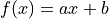 is made to align with a series of xy data points that
have some uncertainty along the x axis and the y axis.
This example demonstrates how to perform such a line fit in kafe2 and
how to extract the results.
is made to align with a series of xy data points that
have some uncertainty along the x axis and the y axis.
This example demonstrates how to perform such a line fit in kafe2 and
how to extract the results.
kafe2go
To run this example, open a text editor and save the following file contents
as a YAML file named line_fit.yml.
# Example 01: Line fit
# In this example a line f(x) = a * x + b is being fitted
# to some data points with pointwise uncertainties.

# The minimal keywords needed to perform a fit are x_data,
# y_data, and y_errors.
# You might also want to define x_errors.

# Data is defined by lists:
x_data: [1.0, 2.0, 3.0, 4.0]

# For errors lists describe pointwise uncertainties.
# By default the errors will be uncorrelated.
x_errors: [0.05, 0.10, 0.15, 0.20]

# Because x_errors is equal to 5% of x_data we could have also defined it like this:
# x_errors: 5%

# In total the following x data will be used for the fit:
# x_0: 1.0 +- 0.05
# x_1: 2.0 +- 0.10
# x_2: 3.0 +- 0.15
# x_3: 4.0 +- 0.20

# In yaml lists can also be written out like this:
y_data:
- 2.3
- 4.2
- 7.5
- 9.4

# The above is equivalent to
# y_data: [2.3, 4.2, 7.5, 9.4]

# For errors a single float gives each data point
# the same amount of uncertainty:
y_errors: 0.4

# The above is equivalent to
# y_errors: [0.4, 0.4, 0.4, 0.4]

# In total the following y data will be used for the fit:
# y_0: 2.3 +- 0.4
# y_1: 4.2 +- 0.4
# y_2: 7.5 +- 0.4
# y_3: 9.4 +- 0.4
Then open a terminal, navigate to the directory where the file is located and run
kafe2go line_fit.yml
Python
The same fit can also be performed by using a Python script.
#!/usr/bin/env python
"""
kafe2 example: Line Fit
=======================

The simplest, and also the most common use case of a fitting framework
is performing a line fit: A linear function of the form
f(x) = a * x + b is made to align with a series of xy data points that
have some uncertainty along the x axis and the y axis.
This example demonstrates how to perform such a line fit in kafe2 and
how to extract the results.
"""

import kafe2

# Define or read in the data for your fit:
x_data = [1.0, 2.0, 3.0, 4.0]
y_data = [2.3, 4.2, 7.5, 9.4]
# x_data and y_data are combined depending on their order.
# The above translates to the points (1.0, 2.3), (2.0, 4.2), (3.0, 7.5), and (4.0, 9.4).

# Important: Specify uncertainties for the data!
x_error = 0.1
y_error = 0.4

# Pass the information to kafe2:
kafe2.xy_fit("line", x_data, y_data, x_error=x_error, y_error=y_error)
# The string "line" gets mapped to a first degree polynomial for the model function.

# Call another function to create a plot:
kafe2.plot(
    x_label="x",  # x axis label
    y_label="y",  # y axis label
    data_label="Data",  # label of data in legend
)

# For backwards compatibility with PhyPraKit kafe2 also has a function k2Fit.
# Internally this method simply uses xy_fit and plot:
# kafe2.k2Fit("line", x_data, y_data, sx=x_error, sy=y_error)
# New code should not use this function!
If you’re performing the fit via Python code there should be two plots. The second plot which shows the so-called profile likelihood (“contour plot”) will be explained in the next chapter.
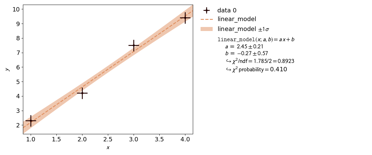
2. Model Functions
In experimental physics a line fit will only suffice for a small number of applications. In most cases you will need a more complex model function with more parameters to accurately model physical reality. This example demonstrates how to specify arbitrary model functions for a kafe2 fit. When a different function has to be fitted, those functions need to be defined either in the YAML file or the Python script.
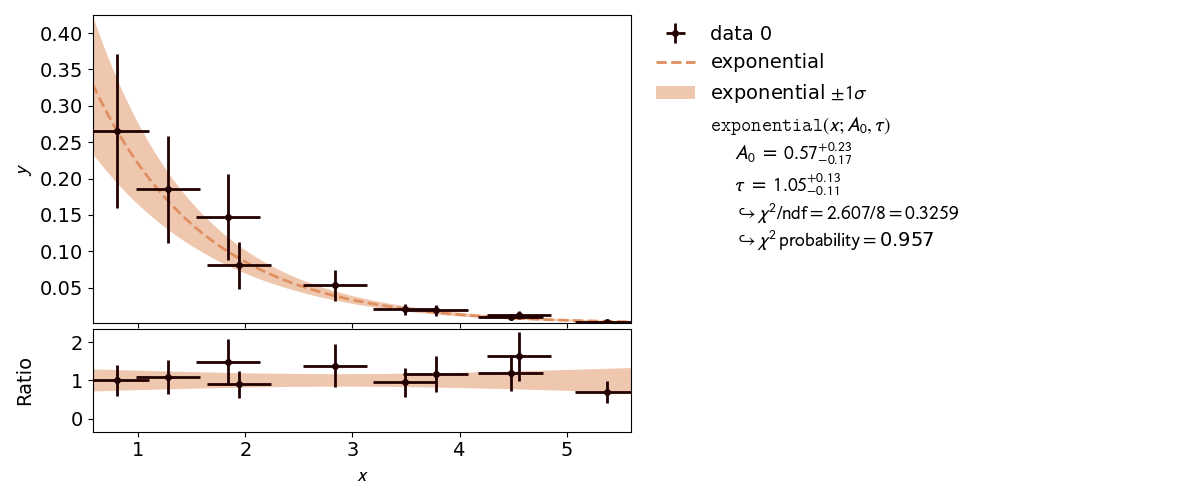
The graphical output itself does not clearly indicate which of the models is acceptable.
For this purpose a hypothesis test can be performed which indicates the so-called  probability - i.e. the probability of obtaining a worse value for at the
minimum than the observed one.
A higher value corresponds to a better fit.
The probability of a fit is shown inside the fit info box on the right.
probability - i.e. the probability of obtaining a worse value for at the
minimum than the observed one.
A higher value corresponds to a better fit.
The probability of a fit is shown inside the fit info box on the right.
An exponential function is a non-linear function!
Non-linear refers to the linearity of the parameters.
Any polynomial like  is a linear function of the parameters
 ,
,  and
and  .
An exponential function
.
An exponential function  is non-linear in its parameter
  .
Thus the profile of can have a non-parabolic shape.
If that is the case, uncertainties of the form
.
Thus the profile of can have a non-parabolic shape.
If that is the case, uncertainties of the form  may not be accurate.
Please refer to 3.1: Profiling for more information.
may not be accurate.
Please refer to 3.1: Profiling for more information.
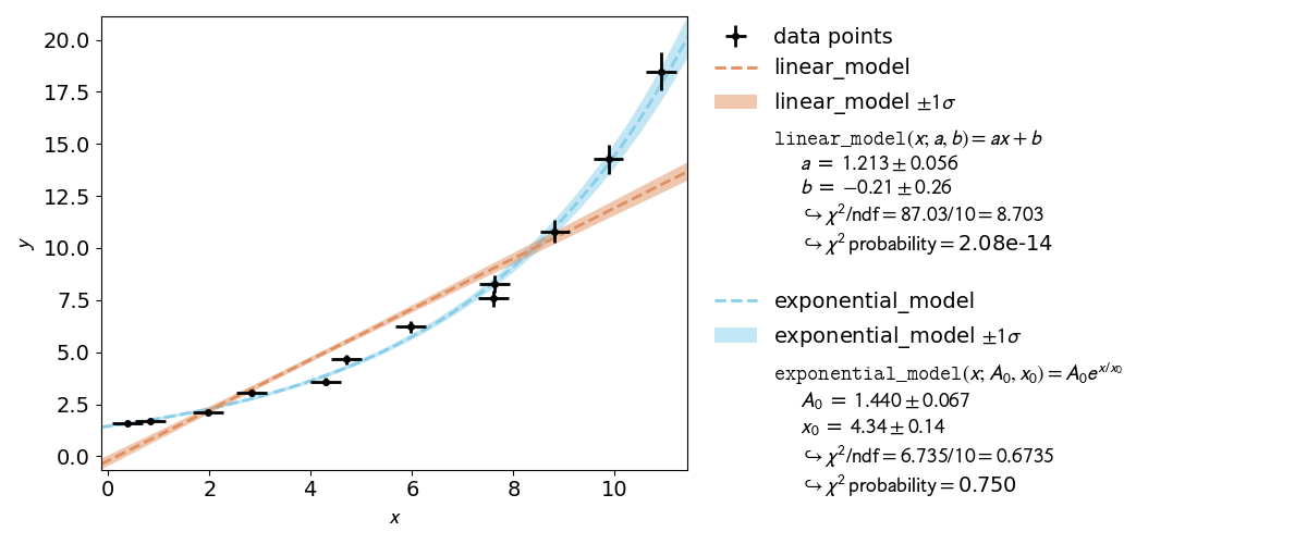
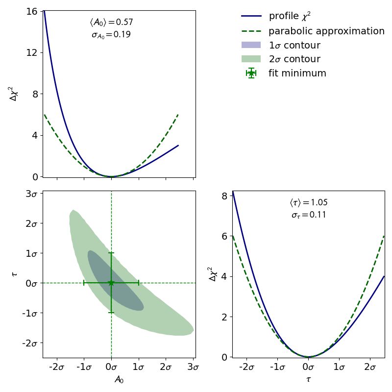
To see the shape of the profiles and contours, please create a contour plot of the fitted
parameters.
This can be done by appending the -c or --contours option to kafe2go.
Additionally a grid can be added to the contour plots with the --grid all flag.
With the simplified Python interface a contour plot is created automatically when x errors or
relative y errors are specified or when setting the keyword argument profile=True.
The object-oriented interface uses the ContoursProfiler object
the usage of which is shown further down.
The corresponding contour plot for the exponential fit shown above looks like this:
When looking at the profiles of the parameters, a deformation is effectively not
present.
In this case the fit results and uncertainties are perfectly fine and are can be used as is.
See 3.1: Profiling for more information.
kafe2go
Inside a YAML file custom fit functions can be defined with the model_function keyword.
The default way to define said model functions is to write a function Python function.
NumPy and SciPy functions are supported without extra import
statements, as shown in the example.
Alternatively model functions can be defined via SymPy (symbolic Python).
The part of the model function left of the string -> is interpreted as SymPy symbols,
the part on the right is interpreted as a SymPy expression using said symbols.
The leftmost part of the string up to : is interpreted as the model function name
(can be omitted).
For more advanced fit functions, consider using kafe2 inside a Python script.
x_data:
- 0.3811286952593707
- 0.8386314422752791
- 1.965701211114396
- 2.823689293793774
- 4.283116179196964
- 4.697874987903564
- 5.971438461333021
- 7.608558039032569
- 7.629881032308029
- 8.818924700702548
- 9.873903963026425
- 10.913590565136278
x_errors:
- correlation_coefficient: 0.0
  error_value: 0.3  # use absolute errors, in this case always 0.3
  relative: false
  type: simple
y_data:
- 1.604521233331755
- 1.6660578688633165
- 2.1251504836493296
- 3.051883842283453
- 3.5790120649006685
- 4.654148130730669
- 6.213711922872129
- 7.576981533273081
- 8.274440603191387
- 10.795366227038528
- 14.272404187046607
- 18.48681513824193
y_errors:
- correlation_coefficient: 0.0
  error_value: 0.05
  relative: true  # use relative errors, in this case 5% of each value
  type: simple

model_function: |
  def exponential_model(x, A_0=1., x_0=5.):
    return A_0 * np.exp(x/x_0)

# If SymPy is installed the model function can also be defined like this:
# model_function: "exponential_model: x A_0 x_0 -> A_0 * exp(x / x_0)"
x_data:
- 0.3811286952593707
- 0.8386314422752791
- 1.965701211114396
- 2.823689293793774
- 4.283116179196964
- 4.697874987903564
- 5.971438461333021
- 7.608558039032569
- 7.629881032308029
- 8.818924700702548
- 9.873903963026425
- 10.913590565136278
x_errors:
- correlation_coefficient: 0.0
  error_value: 0.3  # use absolute errors, in this case always 0.3
  relative: false
  type: simple
y_data:
- 1.604521233331755
- 1.6660578688633165
- 2.1251504836493296
- 3.051883842283453
- 3.5790120649006685
- 4.654148130730669
- 6.213711922872129
- 7.576981533273081
- 8.274440603191387
- 10.795366227038528
- 14.272404187046607
- 18.48681513824193
y_errors:
- correlation_coefficient: 0.0
  error_value: 0.05
  relative: true  # use relative errors, in this case 5% of each value
  type: simple

model_function: |
  def linear_model(x, a=1.0, b=1.0):
      return a * x + b

# If SymPy is installed the model function can also be defined like this:
# model_function: "linear_model: x a b -> a * x + b"
To use multiple input files with kafe2go, simply run
kafe2go path/to/fit1.yml path/to/fit2.yml
To plot the fits in two separate figures append the --separate flag to the kafe2go command.
kafe2go path/to/fit1.yml path/to/fit2.yml --separate
For creating a contour plot, simply add -c to the command line. This will create contour plots
for all given fits.
kafe2go path/to/fit1.yml path/to/fit2.yml --separate -c
Python
When using Python multiple model functions can be defined in the same file.
They are plotted together by first calling kafe2.xy_fit multiple times and then calling
kafe2.plot.
import numpy as np
import kafe2


# To define a model function for kafe2 simply write it as a Python function.
# Important: The first argument of the model function is interpreted as the independent variable
#     of the fit. It is not being modified during the fit and it's the quantity represented by
#     the x axis of our fit.

# Our first model is a simple linear function:
def linear_model(x, a=1.0, b=1.0):
    return a * x + b


# If SymPy is installed you can also define the model like this:
# linear_model = "linear_model: x a=1.0 b=1.0 -> a * x + b"


# Our second model is a simple exponential function.
# The kwargs in the function header specify parameter defaults.
def exponential_model(x, A_0=1.0, x_0=5.0):
    return A_0 * np.exp(x/x_0)


# If SymPy is installed you can also define the model like this:
# exponential_model = "exponential_model: x A_0 x_0=5.0 -> A_0 * exp(x / x_0)"


x_data = [0.38, 0.83, 1.96, 2.82, 4.28, 4.69, 5.97, 7.60, 7.62, 8.81, 9.87, 10.91]
y_data = [1.60, 1.66, 2.12, 3.05, 3.57, 4.65, 6.21, 7.57, 8.27, 10.79, 14.27, 18.48]
x_error = 0.2  # 0.2 in absolute units of x
y_error = 0.5  # 0.5 in absolute units of y
y_error_rel = 0.03  # 3% of the y model value

# kafe2.xy_fit needs to be called twice to do two fits:
kafe2.xy_fit(linear_model, x_data, y_data,
             x_error=x_error, y_error=y_error, y_error_rel=y_error_rel)
kafe2.xy_fit(exponential_model, x_data, y_data,
             x_error=x_error, y_error=y_error, y_error_rel=y_error_rel)
# Make sure to specify profile=True whenever you use a nonlinear model function.
# A model function is linear if it is a linear function of each of its parameters.
# The model function does not need to be a linear function of the independent variable x.
# Examples: all polynomial model functions are linear, trigonometric functions are nonlinear.

# To specify that you want a plot of the last two fits pass -2 as the first argument:
kafe2.plot(
    -2,

    # Uncomment the following line to use different names for the parameters:
    # parameter_names=dict(x="t", a=r"\alpha", b=r"\beta", A_0="I_0", x_0="t_0"),
    # Use LaTeX for special characters like greek letters.

    # When Python functions are used as custom model functions kafe2 does not know
    # how to express them as LaTeX. The LaTeX can be manually defined like this:
    model_expression=["{a}{x} + {b}", "{A_0} e^{{{x}/{x_0}}}"],
    # Parameter names have to be put between {}. To get {} for LaTex double them like {{ or }}.
    # When using SymPy to define model function the LaTeX expression can be derived automatically.

    # Add a so-called pull plot in order to compare the influence of individual data points on the models.
    extra="pull"
    # Alternative extra plots: "residual" or "ratio".
)
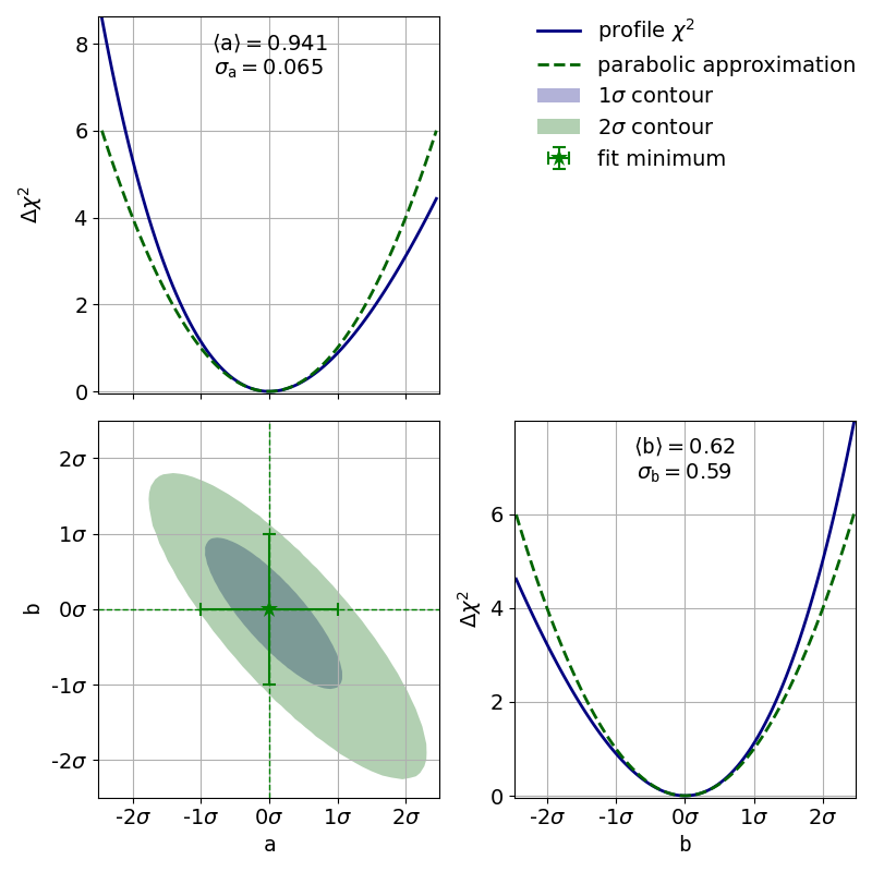
3.1: Profiling
Very often, when the fit model is a non-linear function of the parameters, the
function is not parabolic around the minimum.
A very common example of such a case is an exponential function parametrized as shown in this
example.
In the case of a nonlinear fit, the minimum of a cost function is no longer shaped
like a parabola (with a model parameter on the x axis and on the y axis).
Now, you might be wondering why you should care about the shape of the function.
The reason why it’s important is that the common notation of  for fit results
is only valid for a parabola-shaped cost function.
If your likelihood function is distorted it will also affect your fit results!
for fit results
is only valid for a parabola-shaped cost function.
If your likelihood function is distorted it will also affect your fit results!
Luckily nonlinear fits oftentimes still produce meaningful fit results as long as the distortion is
not too big - you just need to be more careful during the evaluation of your fit results.
A common approach for handling nonlinearity is to trace the profile of the cost function
(in this case ) in either direction of the cost function minimum and find the points
at which the cost function value has increased by a specified amount relative to the cost function
minimum.
In other words, two cuts are made on either side of the cost function minimum at a specified height.
The two points found with this approach span a confidence interval for the fit parameter around the
cost function minimum.
The confidence level of the interval depends on how high you set the cuts for the cost increase
relative to the cost function minimum.
The one sigma interval described by conventional parameter errors is achieved by a cut at the fit
minimum plus  and has a confidence level of about 68%.
The two sigma interval is achieved by a cut at the fit minimum plus
and has a confidence level of about 68%.
The two sigma interval is achieved by a cut at the fit minimum plus  and has a
confidence level of about 95%, and so on.
The one sigma interval is commonly described by what is called asymmetric errors:
the interval limits are described relative to the cost function minimum as
and has a
confidence level of about 95%, and so on.
The one sigma interval is commonly described by what is called asymmetric errors:
the interval limits are described relative to the cost function minimum as
 .
.
In addition to non-linear function, the usage of x data errors leads to a non-linear fits as well. This is shown in 3.3: x-Errors:.
kafe2go
To display asymmetric parameter uncertainties use the flag -a. In addition the profiles and
contours can be shown by using the -c flag. In the Python example a ratio between the data
and model function is shown below the plot. This can be done by appending the -r flag to
kafe2go.
# This is an example for a non-linear fit
# Please run with 'kafe2go -a -c' to show asymmetric uncertainties and the contour profiles

x_data: [0.8018943, 1.839664, 1.941974, 1.276013, 2.839654, 3.488302, 3.775855, 4.555187, 4.477186, 5.376026]
x_errors: 0.3
y_data: [0.2650644, 0.1472682, 0.08077234, 0.1850181, 0.05326301, 0.01984233, 0.01866309, 0.01230001, 0.009694612,
         0.002412357]
y_errors: [0.1060258, 0.05890727, 0.03230893, 0.07400725, 0.0213052, 0.00793693, 0.007465238, 0.004920005, 0.003877845,
           0.0009649427]

model_function: |
  def exponential(x, A_0=1, tau=1):
      return A_0 * np.exp(-x/tau)
Python
From this point on the examples use the object-oriented Python interface. For a quick intorduction consider this code that is mostly equivalent to the very first example of a straight line with xy errors:
from kafe2 import XYContainer, Fit, Plot, ContoursProfiler

# Create an XYContainer object to hold the xy data for the fit:
xy_data = XYContainer(x_data=[1.0, 2.0, 3.0, 4.0],
                      y_data=[2.3, 4.2, 7.5, 9.4])
# x_data and y_data are combined depending on their order.
# The above translates to the points (1.0, 2.3), (2.0, 4.2), (3.0, 7.5), and (4.0, 9.4).

# Important: Specify uncertainties for the data:
xy_data.add_error(axis='x', err_val=0.1)
xy_data.add_error(axis='y', err_val=0.4)

xy_data.label = 'Data'  # How the data is called in plots

# Create an XYFit object from the xy data container.
# By default, a linear function f=a*x+b will be used as the model function.
line_fit = Fit(data=xy_data)

# Perform the fit: Find values for a and b that minimize the
#     difference between the model function and the data.
line_fit.do_fit()  # This will throw a warning if no errors were specified.

# Optional: Print out a report on the fit results on the console.
line_fit.report()
# With kafe2.xy_fit this gets printed to a file.

# Optional: Create a plot of the fit results using Plot.
plot = Plot(fit_objects=line_fit)  # Create a kafe2 plot object.
plot.x_label = 'x'  # Set x axis label.
plot.y_label = 'y'  # Set y axis label.
plot.plot()  # Do the plot.

plot.save()  # Saves the plot to file 'fit.png' .
# plot.save('my_fit.pdf')  # Saves the plot to a different file / with a different file extension.

# Use the ContoursProfiler object to create contour plots:
cpf = ContoursProfiler(line_fit)
cpf.plot_profiles_contours_matrix()

# Show the fit result.
plot.show()  # Just a convenience wrapper for matplotlib.pyplot.show() .
# NOTE: Calling matplotlib.pyplot.show() closes all figures by default so call this AFTER saving.

# Alternatively you could still use the function kafe.plot like this:
# from kafe2 import plot  # Notice that "plot" is not capitalized. "Plot" is the plot object.
# kafe2.plot(line_fit)  # Pass the fit object to the plot function.
Now for the actual example. The relevant lines to display asymmetric uncertainties and to create the contour plot are highlighted in the code example below.
import numpy as np
from kafe2 import Fit, Plot, ContoursProfiler

def exponential(x, A_0=1, tau=1):
    return A_0 * np.exp(-x/tau)

# define the data as simple Python lists
x = [8.018943e-01, 1.839664e+00, 1.941974e+00, 1.276013e+00, 2.839654e+00, 3.488302e+00,
     3.775855e+00, 4.555187e+00, 4.477186e+00, 5.376026e+00]
xerr = 3.000000e-01
y = [2.650644e-01, 1.472682e-01, 8.077234e-02, 1.850181e-01, 5.326301e-02, 1.984233e-02,
     1.866309e-02, 1.230001e-02, 9.694612e-03, 2.412357e-03]
yerr = [1.060258e-01, 5.890727e-02, 3.230893e-02, 7.400725e-02, 2.130520e-02, 7.936930e-03,
        7.465238e-03, 4.920005e-03, 3.877845e-03, 9.649427e-04]

# create a fit object from the data arrays
fit = Fit(data=[x, y], model_function=exponential)
fit.add_error(axis='x', err_val=xerr)  # add the x-error to the fit
fit.add_error(axis='y', err_val=yerr)  # add the y-errors to the fit

fit.do_fit()  # perform the fit
fit.report(asymmetric_parameter_errors=True)  # print a report with asymmetric uncertainties

# Optional: create a plot
plot = Plot(fit)
plot.plot(asymmetric_parameter_errors=True, ratio=True)  # ratio = data / model function

# Optional: create the contours profiler
cpf = ContoursProfiler(fit)
cpf.plot_profiles_contours_matrix()  # plot the contour profile matrix for all parameters

plot.show()
3.2: Double Slit
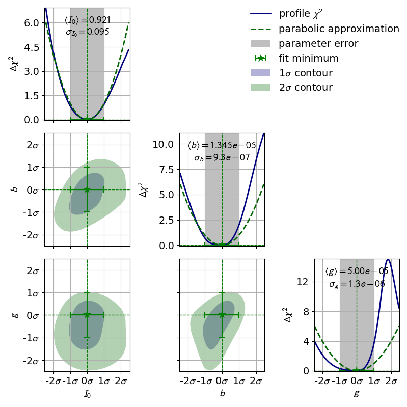
A real world example, when asymmetric parameter uncertainties are needed is the double slit experiment. Here the model function is highly non-linear.
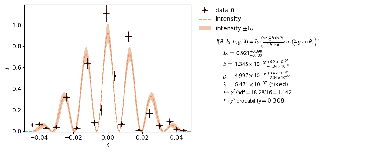
This is also reflected by the highly distorted contours.
kafe2go
A YAML file for this example is available on
GitHub.
It works perfectly fine with kafe2go, but is not edited to a compact form.
It is in fact a direct dump from the fit object used in the python script.
kafe2 supports writing fits and datasets to a kafe2go compatible file with the
data.to_file("my.yml") and fit.to_file("filename.yml") methods as well as
reading them with the corresponding classes like XYContainer.from_file("my.yml") and
XYFit.from_file("filename.yml") as shown in the Python example.
Python
import numpy as np
from kafe2.fit import XYContainer, Fit, Plot
from kafe2.fit.tools import ContoursProfiler


def _generate_dataset(output_filename='02_double_slit_data.yml'):
    """
    Create an XYContainer holding the measurement data
    and the errors and write it to a file.
    """

    xy_data = [[  # x data: position
                -0.044, -0.040, -0.036, -0.030, -0.024, -0.018, -0.012, -0.008, -0.004, -0.001,
                 0.004,  0.008,  0.012,  0.018,  0.024,  0.030,  0.036,  0.040,  0.044],
               [  # y data: light intensity
                0.06, 0.07, 0.03, 0.04, 0.32, 0.03, 0.64, 0.08, 0.20, 1.11, 0.52, 0.07, 0.89, 0.01,
                0.17, 0.05, 0.09, 0.02, 0.01]]

    data = XYContainer(x_data=xy_data[0], y_data=xy_data[1])

    data.add_error('x', 0.002, relative=False, name='x_uncor_err')
    data.add_error(
        'y',
        [0.02, 0.02, 0.02, 0.02, 0.04, 0.02, 0.05, 0.03, 0.05, 0.08, 0.05, 0.03, 0.05, 0.01, 0.04,
         0.03, 0.03, 0.02, 0.01],
        relative=False,
        name='y_uncor_err'
    )

    data.to_file(output_filename)

# Uncomment this to re-generate the dataset:
# _generate_dataset()


def intensity(theta, I_0, b, g, varlambda):
    """
    In this example our model function is the intensity of diffracted light as described by the
    Fraunhofer equation.
    :param theta: angle at which intensity is measured
    :param I_0: intensity amplitude
    :param b: width of a single slit
    :param g: distance between the two slits
    :param varlambda: wavelength of the laser light
    :return: intensity of the diffracted light
    """
    single_slit_arg = np.pi * b * np.sin(theta) / varlambda
    single_slit_interference = np.sin(single_slit_arg) / single_slit_arg
    double_slit_interference = np.cos(np.pi * g * np.sin(theta) / varlambda)
    return I_0 * single_slit_interference ** 2 * double_slit_interference ** 2


# Read in the measurement data from the file generated above:
data = XYContainer.from_file("02_double_slit_data.yml")


# Create fit from data container:
fit = Fit(data=data, model_function=intensity, minimizer="iminuit")

# Optional: assign LaTeX names for prettier fit info box:
fit.assign_model_function_latex_name('I')
fit.assign_model_function_latex_expression(
    r"{I_0}\,\left(\frac{{\sin(\frac{{\pi}}{{{varlambda}}}\,b\,\sin{{{theta}}})}}"
    r"{{\frac{{\pi}}{{{varlambda}}}\,b\,\sin{{{theta}}}}}"
    r"\cos(\frac{{\pi}}{{{varlambda}}}\,g\,\sin{{{theta}}})\right)^2"
)

# Limit parameters to positive values to better model physical reality:
eps = 1e-8
fit.limit_parameter('I_0', lower=eps)
fit.limit_parameter('b', lower=eps)
fit.limit_parameter('g', lower=eps)

# Set fit parameters to near guesses to improve convergence:
fit.set_parameter_values(I_0=1., b=20e-6, g=50e-6)

# The fit parameters have no preference in terms of values.
# Their profiles are highly distorted, indicating a very non-linear fit.
# You can try constraining them via external measurements to make the fit more linear:
# f.add_parameter_constraint('b', value=13.5e-6, uncertainty=1e-6)
# f.add_parameter_constraint('g', value=50e-6, uncertainty=1e-6)

# Fix the laser wavelength to 647.1 nm (krypton laser) since its uncertainty is negligible:
fit.fix_parameter('varlambda', value=647.1e-9)

# Fit objects can also be saved to files:
fit.to_file('02_double_slit.yml')
# The generated file can be used as input for kafe2go.

# Alternatively you could load it back into code via:
# f = XYFit.from_file('02_double_slit.yml')

fit.do_fit()

cpf = ContoursProfiler(fit, contour_cl_values=(0.9, 0.95))
cpf.plot_profiles_contours_matrix(parameters=['I_0', 'b', 'g'],
                                  show_grid_for='all',
                                  show_fit_minimum_for='all',
                                  show_error_span_profiles=True,
                                  show_legend=True,
                                  show_parabolic_profiles=True,
                                  show_ticks_for='all',
                                  contour_naming_convention='cl',
                                  label_ticks_in_sigma = False,
                                  sigma_steps = 1.0)

# To see the fit results, plot using Plot:
p = Plot(fit_objects=fit)
p.y_label = r"$I$"
p.plot(asymmetric_parameter_errors=True)

# Show the fit results:
p.show()
3.3: x-Errors:
In addition to non-linear function, the usage of x data errors leads to a non-linear fits as well.
kafe2 fits support the addition of x data errors - in fact we’ve been using them since the very
first example.
To take them into account the x errors are converted to y errors via multiplication with the
derivative of the model function.
In other words, kafe2 fits extrapolate the derivative of the model function at the x data values
and calculate how a difference in the x direction would translate to the y direction.
Unfortunately this approach is not perfect though.
Since we’re extrapolating the derivative at the x data values, we will only receive valid results
if the derivative doesn’t change too much at the scale of the x error.
Also, since the effective y error has now become dependent on the derivative of the model function
it will vary depending on our choice of model parameters.
This distorts our likelihood function - the minimum of a cost function will no
longer be shaped like a parabola (with a model parameter on the x axis and on the
y axis).
To demonstrate this, the second file x_errors will perform a line fit with much bigger
uncertainties on the x axis than on the y axis. The non-parabolic shape can be seen in the
one-dimensional profile scans.
The effects of this deformation are explained in 3.1: Profiling.
kafe2go
Keep in mind that kafe2go will perform a line fit if no fit function has been specified.
In order do add a grid to the contours, run kafe2go with the --grid all flag.
So to plot with asymmetric errors, the profiles and contour as well as a grid run
kafe2go x_errors.yml -a -c --grid all
# kafe2 XYContainer yaml representation written by johannes on 23.07.2019, 16:57.
type: xy
x_data:
- 0.0
- 1.0
- 2.0
- 3.0
- 4.0
- 5.0
- 6.0
- 7.0
- 8.0
- 9.0
- 10.0
- 11.0
- 12.0
- 13.0
- 14.0
- 15.0
y_data:
- 0.2991126116324785
- 2.558050235697161
- 1.2863728164289798
- 3.824686039107114
- 2.843373362329926
- 5.461953737679532
- 6.103072604470123
- 8.166562633164254
- 8.78250807001851
- 8.311966900704014
- 8.980727588512268
- 11.144142620167695
- 11.891326143534158
- 12.126133797209802
- 15.805993018808897
- 15.3488445186788
# The x errors are much bigger than the y errors. This will strongly distort the likelihood function.
x_errors: 1.0
y_errors: 0.1
Python
The example to show that uncertainties on the x axis can cause a non-linear fit uses the YAML dataset given in the kafe2go section.
from kafe2 import XYContainer, Fit, Plot
from kafe2.fit.tools import ContoursProfiler

# Construct a fit with data loaded from a yaml file. The model function is the default of f(x) = a * x + b
nonlinear_fit = Fit(data=XYContainer.from_file('03_x_errors.yml'))

# The x errors are much bigger than the y errors. This will cause a distortion of the likelihood function.
nonlinear_fit.add_error('x', 1.0)
nonlinear_fit.add_error('y', 0.1)

# Perform the fit.
nonlinear_fit.do_fit()

# Optional: Print out a report on the fit results on the console.
# Note the asymmetric_parameter_errors flag
nonlinear_fit.report(asymmetric_parameter_errors=True)

# Optional: Create a plot of the fit results using Plot.
# Note the asymmetric_parameter_errors flag
plot = Plot(nonlinear_fit)
plot.plot(fit_info=True, asymmetric_parameter_errors=True)

# Optional: Calculate a detailed representation of the profile likelihood
# Note how the actual chi2 profile differs from the parabolic approximation that you would expect with a linear fit.
profiler = ContoursProfiler(nonlinear_fit)
profiler.plot_profiles_contours_matrix(show_grid_for='all')

plot.show()
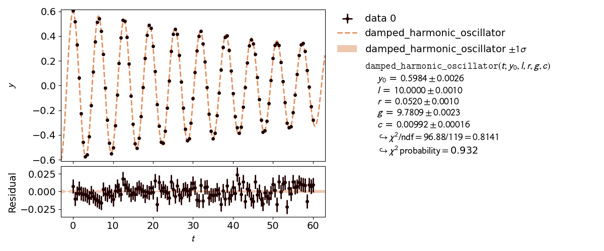
4: Constraints
The models used to describe physical phenomena usually depend on a multitude of parameters. However, for many experiments only one of the parameters is of actual interest to the experimenter. Still, because model parameters are generally not uncorrelated the experimenter has to factor in the nuisance parameters for their estimation of the parameter of interest.
Historically this has been done by propagating the uncertainties of the nuisance parameters onto the y-axis of the data and then performing a fit with those uncertainties. Thanks to computers, however, this process can also be done numerically by applying parameter constraints. This example demonstrates the usage of those constraints in the kafe2 framework.
More specifically, this example will simulate the following experiment:
A steel ball of radius  has been connected to the ceiling by a string of length
  ,
forming a pendulum. Due to earth’s gravity providing a restoring force this system is a harmonic
oscillator. Because of friction between the steel ball and the surrounding air the oscillator is
also damped by the viscous damping coefficient .
,
forming a pendulum. Due to earth’s gravity providing a restoring force this system is a harmonic
oscillator. Because of friction between the steel ball and the surrounding air the oscillator is
also damped by the viscous damping coefficient .
The goal of the experiment is to determine the local strength of earth’s gravity  . Since
the earth is shaped like an ellipsoid the gravitational pull varies with latitude: it’s strongest
at the poles with
. Since
the earth is shaped like an ellipsoid the gravitational pull varies with latitude: it’s strongest
at the poles with 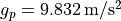 and it’s weakest at the equator with
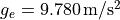 . For reference, at Germany’s latitude lies at
approximately
. For reference, at Germany’s latitude lies at
approximately  .
.
kafe2go
Parameter constraints are straightforward to use with kafe2go. After defining the model function parameter constraints can be set. Simple gaussian constraints can be defined with the parameter name followed by the required information as highlighted in the example. For more information on parameter constraints via a covariance matrix, please refer to Parameter Constraints.
x_data: [0.0, 0.5, 1.0, 1.5, 2.0, 2.5, 3.0, 3.5, 4.0, 4.5, 5.0, 5.5, 6.0, 6.5, 7.0, 7.5, 8.0, 8.5,
         9.0, 9.5, 10.0, 10.5, 11.0, 11.5, 12.0, 12.5, 13.0, 13.5, 14.0, 14.5, 15.0, 15.5, 16.0,
         16.5, 17.0, 17.5, 18.0, 18.5, 19.0, 19.5, 20.0, 20.5, 21.0, 21.5, 22.0, 22.5, 23.0, 23.5,
         24.0, 24.5, 25.0, 25.5, 26.0, 26.5, 27.0, 27.5, 28.0, 28.5, 29.0, 29.5, 30.0, 30.5, 31.0,
         31.5, 32.0, 32.5, 33.0, 33.5, 34.0, 34.5, 35.0, 35.5, 36.0, 36.5, 37.0, 37.5, 38.0, 38.5,
         39.0, 39.5, 40.0, 40.5, 41.0, 41.5, 42.0, 42.5, 43.0, 43.5, 44.0, 44.5, 45.0, 45.5, 46.0,
         46.5, 47.0, 47.5, 48.0, 48.5, 49.0, 49.5, 50.0, 50.5, 51.0, 51.5, 52.0, 52.5, 53.0, 53.5,
         54.0, 54.5, 55.0, 55.5, 56.0, 56.5, 57.0, 57.5, 58.0, 58.5, 59.0, 59.5, 60.0]
x_errors: 0.001

y_data: [0.6055317575993914, 0.5169107902610475, 0.3293169273559535, 0.06375859733814328,
         -0.22640917641452488, -0.4558011426302008, -0.5741274235093591, -0.5581292464350779,
         -0.4123919729458466, -0.16187396188197636, 0.11128294449725282, 0.3557032748758762,
         0.5123991632742368, 0.5426212570679745, 0.441032201346871, 0.2530635717934812,
         -0.018454841476861578, -0.27767282674995675, -0.4651897678670606, -0.5496969201663507,
         -0.5039723480612176, -0.32491507193649194, -0.07545061334934718, 0.17868596924060803,
         0.38816743920465974, 0.5307390166315159, 0.5195411750524918, 0.3922352276601664,
         0.1743316249378316, -0.08489324112691513, -0.31307737388477896, -0.47061848549403956,
         -0.5059137659253059, -0.4255733083473707, -0.24827692102709906, -0.013334081799533964,
         0.21868390151118114, 0.40745363855032496, 0.4900638626421252, 0.4639947376885959,
         0.3160179896333209, 0.11661884242058931, -0.15370888958327286, -0.32616191426973545,
         -0.45856921225721586, -0.46439857887558106, -0.3685539265001533, -0.1830244989818371,
         0.03835530881316253, 0.27636300051486506, 0.4163001580121898, 0.45791960756716926,
         0.4133277046353799, 0.2454571744527809, 0.02843505139404641, -0.17995259849041545,
         -0.3528170613993332, -0.4432670688586229, -0.4308872405896063, -0.3026153676925856,
         -0.10460001285649327, 0.10576999137260902, 0.2794125634785019, 0.39727960494083775,
         0.44012013094335295, 0.33665573392945614, 0.19241116925921273, -0.01373255454051425,
         -0.2288093781464643, -0.36965277845455136, -0.4281953074871928, -0.3837254105792804,
         -0.2439384794237307, -0.05945292033865969, 0.12714573185667402, 0.31127632080817996,
         0.38957820781361946, 0.4022425989547513, 0.2852587536434507, 0.12097975879552739,
         -0.06442727622110235, -0.25077071692351, -0.3414562050547135, -0.3844271968533089,
         -0.3344326061358699, -0.1749451011511041, -0.016716872087832926, 0.18543436492361495,
         0.322914548974734, 0.37225887677620817, 0.3396788239855797, 0.254332254048965,
         0.0665429944525343, -0.11267963115652598, -0.2795347352658008, -0.37651751469292644,
         -0.3654799155251143, -0.28854786660062454, -0.14328549945642755, 0.04213065692623846,
         0.2201386996949766, 0.32591680654151617, 0.3421258708802321, 0.32458251078266503,
         0.18777342536595865, 0.032971092778669095, -0.13521542014013244, -0.3024666212766573,
         -0.34121930021830144, -0.33201664443451445, -0.21960116119767256, -0.07735846981040519,
         0.09202435934084172, 0.24410808130924241, 0.3310159788871507, 0.34354629209994936,
         0.2765230394100408, 0.12467034370454594, -0.012680322294530635, -0.1690136862958978,
         -0.27753009059653394]
y_errors: 0.01

# Because the model function is oscillating the fit needs to be initialized with near guesses for
# unconstrained parameters in order to converge.
# To use starting values for the fit, specify them as default values in the fit function.
model_function: |
    def damped_harmonic_oscillator(theta, y_0=1.0, l=1.0, r=1.0, g=9.81, c=0.01):
        # Model function for a pendulum as a 1d, damped harmonic oscillator with zero initial speed
        # x = time, y_0 = initial_amplitude, l = length of the string,
        # r = radius of the steel ball, g = gravitational acceleration, c = damping coefficient
        # effective length of the pendulum = length of the string + radius of the steel ball
        l_total = l + r
        omega_0 = np.sqrt(g / l_total)  # phase speed of an undamped pendulum
        omega_d = np.sqrt(omega_0 ** 2 - c ** 2)  # phase speed of a damped pendulum
        return y_0 * np.exp(-c * theta) * (np.cos(omega_d * theta) + c / omega_d * np.sin(omega_d * theta))

parameter_constraints:    # add parameter constraints
  l:
    value: 10.0
    uncertainty: 0.001    # l = 10.0+-0.001
  r:
    value: 0.052
    uncertainty: 0.001    # r = 0.052+-0.001
  y_0:
    value: 0.6
    uncertainty: 0.006
    relative: true        # Make constraint uncertainty relative to value, y_0 = 0.6+-0.6%
Python
Using kafe2 inside a Python script, parameter constraints can be set with
fit.add_parameter_constraint(). The according section is highlighted in the code example below.
import numpy as np

from kafe2 import XYContainer, Fit, Plot

# Relevant physical magnitudes and their uncertainties:
l, delta_l = 10.0, 0.001  # length of the string, l = 10.0+-0.001 m
r, delta_r = 0.052, 0.001  # radius of the steel ball, r = 0.052+-0.001 m
# Amplitude of the steel ball at t=0 in degrees, y_0 = 0.6+-0.006% degrees:
y_0, delta_y_0 = 0.6, 0.01  # Note that the uncertainty on y_0 is relative to y_0
g_0 = 9.81  # Initial guess for g


# Model function for a pendulum as a 1d, damped harmonic oscillator with zero initial speed:
# t = time, y_0 = initial_amplitude, l = length of the string,
# r = radius of the steel ball, g = gravitational acceleration, c = damping coefficient.
def damped_harmonic_oscillator(t, y_0, l, r, g, c):
    # Effective length of the pendulum = length of the string + radius of the steel ball:
    l_total = l + r
    omega_0 = np.sqrt(g / l_total)  # Phase speed of an undamped pendulum.
    omega_d = np.sqrt(omega_0 ** 2 - c ** 2)  # Phase speed of a damped pendulum.
    return y_0 * np.exp(-c * t) * (np.cos(omega_d * t) + c / omega_d * np.sin(omega_d * t))


# Load data from yaml, contains data and errors:
data = XYContainer.from_file(filename='data.yml')

# Create fit object from data and model function:
fit = Fit(data=data, model_function=damped_harmonic_oscillator)

# Constrain model parameters to measurements:
fit.add_parameter_constraint(name='l',   value=l,   uncertainty=delta_l)
fit.add_parameter_constraint(name='r',   value=r,   uncertainty=delta_r)
fit.add_parameter_constraint(name='y_0', value=y_0, uncertainty=delta_y_0, relative=True)

# Lengths between two points are by definition positive, this can be expressed with one-sided limit.
# Note: for technical reasons these limits are inclusive.
fit.limit_parameter("y_0", lower=1e-6)
fit.limit_parameter("l", lower=1e-6)
fit.limit_parameter("r", lower=1e-6)

# Set limits for g that are much greater than the expected deviation but still close to 9.81:
fit.limit_parameter("g", lower=9.71, upper=9.91)

# Solutions are real if c < g / (l + r). Set the upper limit for c a little lower:
c_max = 0.9 * g_0 / (l + r)
fit.limit_parameter("c", lower=1e-6, upper=c_max)

# Optional: Set the initial values of parameters to our initial guesses.
# This can help with convergence, especially when no constraints or limits are specified.
fit.set_parameter_values(y_0=y_0, l=l, r=r, g=g_0)
# Note: this could also be achieved by changing the positional arguments of our model function
# into keyword arguments with our initial guesses as the default values.

# Perform the fit:
fit.do_fit()

# Optional: Print out a report on the fit results on the console.
fit.report(asymmetric_parameter_errors=True)

# Optional: plot the fit results.
plot = Plot(fit)
plot.plot(residual=True, asymmetric_parameter_errors=True)

plot.show()
5: Convenience
This part includes examples, designed to be used as cheat sheets.
Plot Customization
This example is a cheat sheet for plot/report customization. It briefly demonstrates methods that modify the optics of kafe2 output.
from kafe2 import XYContainer, Fit, Plot

# The same setup as in 001_line_fit/line_fit.py :
xy_data = XYContainer(x_data=[1.0, 2.0, 3.0, 4.0],
                      y_data=[2.3, 4.2, 7.5, 9.4])
xy_data.add_error(axis='x', err_val=0.1)
xy_data.add_error(axis='y', err_val=0.4)
line_fit = Fit(data=xy_data)
line_fit.do_fit()

# Non-LaTeX names are used in reports and other text-based output:
line_fit.assign_parameter_names(x='t', a='alpha', b='beta')
line_fit.assign_model_function_name('theta')
line_fit.assign_model_function_expression("{a} * {x} + {b}")
# Note: the model function expression is formatted as a Python string.
#    The names of parameters in curly brackets will be replaced with the specified latex names.

# You could also just hard-code the parameter names like this:
# line_fit.assign_model_function_expression("alpha * t + beta")

line_fit.report()

# LaTeX names are used in plot info boxes:
line_fit.assign_parameter_latex_names(x='t', a='\\alpha', b='\\beta')
line_fit.assign_model_function_latex_name('\\theta')
line_fit.assign_model_function_latex_expression('{a} \\cdot {x} + {b}')

# Labels can be set for a fit.
# These labels are then used by all Plots created from said fit.
# If a Plot object also defines labels those labels override the fit labels.

# The labels displayed in the info box:
line_fit.data_container.label = "My data label"
line_fit.model_label = "My model label"

# The labels displayed on the x/y axes:
line_fit.data_container.axis_labels = ["My x axis", "My y axis"]

plot = Plot(fit_objects=line_fit)

# Plot objects can be modified with the customize method which sets matplotlib keywords.
# The first argument specifies the subplot for which to set keywords.
# The second argument specifies which keyword to set.
# The third argument is a list of values to set for the keyword for each fit managed
#     by the plot object.

plot.customize('data', 'label', "My data label 2")  # Overwrite data label in info box.
# plot.customize('data', 'label', None)  # Hide data label in info box.
plot.customize('data', 'marker', 'o')  # Set the data marker shape in the plot.
plot.customize('data', 'markersize', 5)  # Set the data marker size in the plot.
plot.customize('data', 'color', 'blue')  # Set the data marker color in the plot.
plot.customize('data', 'ecolor', 'gray')  # Set the data errorbar color in the plot.

plot.customize('model_line', 'label', 'My model label 2')  # Set the model label in the info box.
# plot.customize('model_line', 'label', None)  # Hide the model label in the info box.
plot.customize('model_line', 'color', 'lightgreen')  # Set the model line color in the plot.
plot.customize('model_line', 'linestyle', '-')  # Set the style of the model line in the plot.
plot.customize('model_error_band', 'label', r'$\pm 1 \sigma$')  # Error band label in info box.
# plot.customize('model_error_band', 'label', None)  # Hide error band label.
plot.customize('model_error_band', 'color', 'lightgreen')  # Error band color in plot.
# plot.customize('model_error_band', 'hide', True)  # Hide error band in plot and info box.

# Available keywords can be retrieved with Plot.get_keywords(subplot_type) .
# subplot_type is for example 'data', 'model_line', or 'model_error_band'.

# In addition to the customize method Plot has a few convenience methods for common operations:

plot.x_range = (0.8, 6)  # Set the x range of the plot.
plot.y_range = (1, 11)  # Set the y range of the plot.

plot.x_label = 'My x axis 2'  # Overwrite the label of the x axis.
plot.y_label = 'My y axis 2'  # Overwrite the label of the y axis.

plot.x_scale = 'log'  # Set the x axis to a logarithmic scale.
plot.y_scale = 'log'  # Set the y axis to a logarithmic scale.

# Finally, perform the plot:
plot.plot(ratio=True)
plot.show()
Accessing Fit Data via Properties
In the previous kafe2 examples we retrieved kafe2 results in a human-readable form via reports and plots. This example demonstrates how these fit results can instead be retrieved as Python variables.
from kafe2 import XYContainer, Fit

# The same setup as in 001_line_fit/line_fit.py :
xy_data = XYContainer(x_data=[1.0, 2.0, 3.0, 4.0],
                      y_data=[2.3, 4.2, 7.5, 9.4])
xy_data.add_error(axis='x', err_val=0.1)
xy_data.add_error(axis='y', err_val=0.4)
line_fit = Fit(data=xy_data)

# First option: retrieve the fit results from the dictionary returned by do_fit.
result_dict = line_fit.do_fit()
# This dictionary contains the same information that would be shown in a report or plot.
# It can also be retrieved via
# result_dict = line_fit.get_result_dict()

# Print contents of result dict:
for key in result_dict:
    if "mat" in key:
        print("%s:" % key)
        print(result_dict[key])
    else:
        print("%s = %s" % (key, result_dict[key]))
    print()
# Note: the asymmetric parameter errors are None because computing them is relatively expensive.
# To calculate them run
# result_dict = line_fit.do_fit(asymmetric_parameter_errors=True)
# or
# result_dict = line_fit.get_result_dict(asymmetric_parameter_errors=True)

# A comparable output to above can be achieved by manually calling and printing fit properties:
print("============ Manual prints below ============")
print()
print("did_fit = %s\n" % line_fit.did_fit)
print("cost = %s\n" % line_fit.cost_function_value)
print("ndf = %s\n" % line_fit.ndf)
print("goodness_of_fit = %s\n" % line_fit.goodness_of_fit)
print("gof/ndf = %s\n" % (line_fit.goodness_of_fit / line_fit.ndf))
print("chi2_probability = %s\n" % line_fit.chi2_probability)
print("parameter_values = %s\n" % line_fit.parameter_values)
print("parameter_name_value_dict = %s\n" % line_fit.parameter_name_value_dict)
print("parameter_cov_mat:\n%s\n" % line_fit.parameter_cov_mat)
print("parameter_errors = %s\n" % line_fit.parameter_errors)
print("parameter_cor_mat:\n%s\n" % line_fit.parameter_cor_mat)
print("asymmetric_parameter_errors:\n%s\n" % line_fit.asymmetric_parameter_errors)
Saving Fits
Most kafe2 objects can be turned into the human-readable YAML format and written to a file. These files can then be used to load the objects into Python code or as input for kafe2go.
from kafe2 import XYContainer, XYFit, Fit, Plot

# The same data as in 001_line_fit/line_fit.py :
xy_data = XYContainer(x_data=[1.0, 2.0, 3.0, 4.0],
                      y_data=[2.3, 4.2, 7.5, 9.4])
xy_data.add_error(axis='x', err_val=0.1)
xy_data.add_error(axis='y', err_val=0.4)

# Save the data container to a file:
xy_data.to_file("data_container.yml")
# Because a data container does not have a model function running kafe2go with this file as input
#     will fit a linear model a * x + b .


def quadratic_model(x, a=1.0, b=1.0, c=1.0):
    return a * x ** 2 + b * x + c


line_fit = Fit(data=xy_data, model_function=quadratic_model)

# Save the fit to a file:
line_fit.to_file("fit_before_do_fit.yml")
# Because the fit object contains a model function running kafe2go with this file as input will
#     make use of the model function we defined above.
#
# Note: The context in which the model function is defined is NOT saved. If your model function
#       depends on things outside the function block it cannot be loaded back (NumPy and SciPy
#       are available in the context in which the function is being loaded though).

line_fit.do_fit()

# Save the fit with fit results to a file:
line_fit.to_file("fit_after_do_fit.yml")

# Alternatively we could save only the state (parameter values + fit results) to a file:
line_fit.save_state("fit_results.yml")

# Load it back into code:
loaded_fit = XYFit.from_file("fit_after_do_fit.yml")
# Note: this requires the use of a specific fit class like XYFit. The generic Fit pseudo-class
#     does NOT work.

# Alternatively we could have created a new fit and loaded the fit results:
# loaded_fit = Fit(data=xy_data, model_function=quadratic_model)
# loaded_fit.load_state("fit_results.yml")
#
# Note: Because we defined the model function in regular Python code there are no problems with
#       the context in that it's being defined.

loaded_fit.report()

plot = Plot(fit_objects=loaded_fit)

plot.plot()
plot.show()
6.1: Covariance matrix
kafe2go
type: indexed
data:
- 80.429
- 80.339
- 80.217
- 80.449
- 80.477
- 80.310
- 80.324
- 80.353
errors:
- - 0.055
  - 0.073
  - 0.068
  - 0.058
  - 0.069
  - 0.091
  - 0.078
  - 0.068
- type: matrix
  matrix_type: covariance
  matrix: [[0.000441, 0.000441, 0.000441, 0.000441, 0.000625, 0.000625, 0.000625, 0.000625],
           [0.000441, 0.000441, 0.000441, 0.000441, 0.000625, 0.000625, 0.000625, 0.000625],
           [0.000441, 0.000441, 0.000441, 0.000441, 0.000625, 0.000625, 0.000625, 0.000625],
           [0.000441, 0.000441, 0.000441, 0.000441, 0.000625, 0.000625, 0.000625, 0.000625],
           [0.000625, 0.000625, 0.000625, 0.000625, 0.001936, 0.001936, 0.001936, 0.001936],
           [0.000625, 0.000625, 0.000625, 0.000625, 0.001936, 0.001936, 0.001936, 0.001936],
           [0.000625, 0.000625, 0.000625, 0.000625, 0.001936, 0.001936, 0.001936, 0.001936],
           [0.000625, 0.000625, 0.000625, 0.000625, 0.001936, 0.001936, 0.001936, 0.001936]]
model_function: |
    def average(a):
        # our model is a simple constant function
        return a
Python
import numpy as np
from kafe2 import IndexedContainer, Fit, Plot

measurements = np.array([5.3, 5.2, 4.7, 4.8])  # The results we want to average.
err_stat = 0.2  # Statistical uncertainty for each measurement.
err_syst_1234 = 0.15  # Systematic uncertainty that affects all measurements.
err_syst_12 = 0.175  # Systematic absolute uncertainty only affecting the first two measurements.
err_syst_34 = 0.05  # Systematic relative uncertainty affecting only the last two measurements.

# Create an IndexedContainer from our data:
data = IndexedContainer(measurements)

# Start with an empty matrix for our covariance matrix:
covariance_matrix = np.zeros(shape=(4, 4))
# Uncorrelated uncertainties only affect the diagonal of the covariance matrix:
covariance_matrix += np.eye(4) * err_stat ** 2
# Fully correlated uncertainties that affect all measurements affect all covariance matrix entries:
covariance_matrix += err_syst_1234 ** 2
# Fully correlated uncertainties that affect only a part of the measurements result in block-like
# changes to the covariance matrix:
covariance_matrix[0:2, 0:2] += err_syst_12 ** 2  # Magnitude of abs. uncertainty is the same.
err_syst_34_abs = err_syst_34 * measurements[2:4]  # Magnitude of abs. uncertainty is different.
covariance_matrix[2:4, 2:4] += np.outer(err_syst_34_abs, err_syst_34_abs)

# The covariance matrix can now be simply added to our container to specify the uncertainties:
data.add_matrix_error(covariance_matrix, matrix_type="cov")

# To get the same result we could have also added the uncertainties one-by-one like this:
# data.add_error(err_stat, correlation=0)
# data.add_error(err_syst_1234, correlation=1)
# data.add_error([err_syst_12, err_syst_12, 0, 0], correlation=1)
# data.add_error([0, 0, err_syst_34, err_syst_34], correlation=1, relative=True)
# See the next example for another demonstration of this approach.


# Just for graphical output:
data.label = 'Test data'
data.axis_labels = [None, 'Measured value (a.o.)']


# The very simple "model":
def average(a=5.0):
    return a


# Set up the fit:
fit = Fit(data, average)
fit.model_label = 'average value'

# Perform the fit:
fit.do_fit()

# Report and plot results:
fit.report()
p = Plot(fit)
p.plot()

p.show()
6.2: Error components
Typically, the uncertainties of the measurement data are much more complex than in the examples discussed so far. In most cases there are uncertainties in ordinate and abscissa, and in addition to the independent uncertainties of each data point there are common, correlated uncertainties for all of them.
With the method add_error() or add_matrix_error() uncertainties can be specified on
the ‘x’ and ‘y’ data, either in the form of independent or correlated, relative or absolute
uncertainties of all or groups of measured values or by specifying the complete covariance or
correlation matrix.
All uncertainties specified in this way are included in the global covariance matrix for the fit.
As an example, we consider measurements of a cross section as a function of the energy near a
resonance.
These are combined measurement data from the four experiments at CERN’s LEP accelerator,
which were corrected for effects caused by photon radiation: Measurements of the hadronic cross
section ( ) as a function of the centre-of-mass energy (
 ).
).
Python
from kafe2 import XYContainer, Fit, Plot, ContoursProfiler

# Center-of-mass energy E (GeV):
E = [88.387, 89.437, 90.223, 91.238, 92.059, 93.004, 93.916]  # x data
E_errors = [0.005, 0.0015, 0.005, 0.003, 0.005, 0.0015, 0.005]  # Uncorrelated absolute x errors
ECor_abs = 0.0017  # Correlated absolute x error

# Hadronic cross section with photonic corrections applied (nb):
sig = [6.803, 13.965, 26.113, 41.364, 27.535, 13.362, 7.302]  # y data
sig_errors = [0.036, 0.013, 0.075, 0.010, 0.088, 0.015, 0.045]  # Uncorrelated absolute y errors
sigCor_rel = 0.0007  # Correlated relative y error


# Breit-Wigner with s-dependent width:
def BreitWigner(E, s0=41.0, M_Z=91.2, G_Z=2.5):
    s = E*E
    Msq = M_Z*M_Z
    Gsq = G_Z*G_Z
    return s0*s*Gsq/((s-Msq)*(s-Msq)+(s*s*Gsq/Msq))


BW_data = XYContainer(E, sig)  # Create data container.

# Add errors to data container.
# By default errors are assumed to be absolute and uncorrelated.
# For errors that are relative and/or correlated you need to set the corresponding kwargs.

# Add independent errors:
error_name_sig = BW_data.add_error(axis='x', name='deltaSig', err_val=E_errors)
error_name_E = BW_data.add_error(axis='y', name='deltaE', err_val=sig_errors)

# Add fully correlated, absolute Energy errors:
error_name_ECor = BW_data.add_error(axis='x', name='Ecor', err_val=ECor_abs, correlation=1.)

# Add fully correlated, relative cross section errors:
error_name_sigCor = BW_data.add_error(
    axis='y', name='sigCor', err_val=sigCor_rel, correlation=1., relative=True)

# Note: kafe2 methods that add errors return a name for the added error. If no name is specified
# a random alphanumeric string is assigned automatically. Further down we will use these names to
# enable/disable some of the errors.

# Assign labels for the data and the axes:
BW_data.label = 'QED-corrected hadronic cross-sections'
BW_data.axis_labels = ('CM Energy (GeV)', r'$\sigma_h$ (nb)')
# Note: Because kafe2 containers are copied when a Fit object is created from them assigning labels
# to the original XYContainer after the fit has already been created would NOT work.

model_function = "BreitWigner: x s0=41.0 M_Z=91.2 G_Z=2.5 -> s0 * x^2 * G_Z^2 / ((x^2 - M_Z^2)^2 + x^4 * G_Z^2 / M_Z^2)"
# model_function = BreitWigner  # Uncomment to define the model function in Python code, loses automatic LaTeX.

BW_fit = Fit(BW_data, model_function)

# Uncomment the following two lines to assign data labels after the fit has already been created:
# BW_fit.data_container.label = 'QED-corrected hadronic cross-sections'
# BW_fit.data_container.axis_labels = ('CM Energy (GeV)', r'$\sigma_h$ (nb)')

# Model labels always have to be assigned after the fit has been created:
BW_fit.model_label = 'Beit-Wigner with s-dependent width'

# Set LaTeX names for printout in info-box:
BW_fit.assign_parameter_latex_names(x='E', s0=r'\sigma^0')

# Do the fit:
BW_fit.do_fit()

# Print a report:
BW_fit.report(asymmetric_parameter_errors=True)

# Plot the fit results:
BW_plot = Plot(BW_fit)
BW_plot.y_range = (0, 1.03*max(sig))  # Explicitly set y_range to start at 0.
BW_plot.plot(residual=True, asymmetric_parameter_errors=True)

# Create a contour plot:
ContoursProfiler(BW_fit).plot_profiles_contours_matrix(show_grid_for='contours')

# Investigate the effects of individual error components: disabling the correlated uncertainty on
# energy should decrease the uncertainty of the mass M but have little to no effect otherwise.
print('====== Disabling error component %s ======' % error_name_ECor)
print()
BW_fit.disable_error(error_name_ECor)
BW_fit.do_fit()
BW_fit.report(show_data=False, show_model=False)

BW_plot.show()
6.3: Relative uncertainties
We had already seen that kafe2 allows the declaration of relative uncertainties which we want to examine more closely in this example. Adjustments with relative uncertainties suffer from the fact that the estimate of the parameter values is distorted. This is because measured values that fluctuate to smaller values have smaller uncertainties; the uncertainties are correspondingly greater when the measured values fluctuate upwards. If the random fluctuations were exactly the other way round, other uncertainties would be assigned. It would be correct to relate the relative uncertainties to the true values, which we do not know. Instead, the option reference=’model’ allows the uncertainties to be dependent on the model value - still not completely correct, but much better.
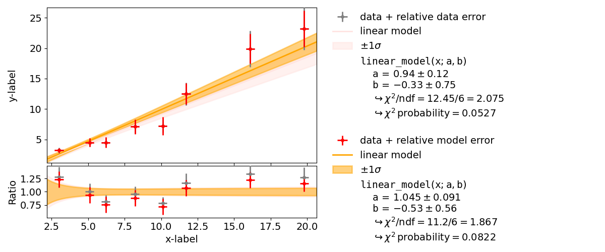
As seen in the example, the probability improves from around  to
to
 and
and  improves from
  to
to  .
.
kafe2go
For using uncertainties relative to the model, The parametric_model section must be added
inside the YAML file, as highlighted below.
For comparison, one cane move the y-uncertainty out of the parametric_model section.
Then the uncertainty will be relative to the data.
# This line fit uses uncertainties relative to the model.
# This requires a little bit more user input, but is still very straightforward.

x_data: [19.8, 3.0, 5.1, 16.1, 8.2, 11.7, 6.2, 10.1]
y_data: [23.2, 3.2, 4.5, 19.9, 7.1, 12.5, 4.5, 7.2]
x_errors: 0.3
label: data + relative model error
x_label: x-label
y_label: y-label

# In order to define uncertainties relative to the model, a parametric model section must be added.
parametric_model:
  model_function: linear_model
  model_label: linear model
  y_errors: 15%
Python
Referencing the model as source for relative uncertainties is done by setting the keyword
reference='model' in the add_error method.
from kafe2 import XYContainer, Fit, Plot, ContoursProfiler

x = [19.8, 3.0, 5.1, 16.1, 8.2,  11.7, 6.2, 10.1]
y = [23.2, 3.2, 4.5, 19.9, 7.1, 12.5, 4.5, 7.2]
data = XYContainer(x_data=x, y_data=y)
data.add_error(axis='x', err_val=0.3)
data.axis_labels = ['x-label', 'y-label']

# create fit with relative data uncertainty
linear_fit1 = Fit(data, model_function='linear_model')
linear_fit1.add_error('y', 0.15, relative=True, reference='data')
linear_fit1.data_container.label = "data + relative data error"
linear_fit1.model_label = "linear model"
linear_fit1.do_fit()

# create fit with relative model uncertainty
linear_fit2 = Fit(data, model_function='linear_model')
linear_fit2.add_error('y', 0.15, relative=True, reference='model')
linear_fit2.data_container.label = "data + relative model error"
linear_fit2.model_label = "linear model"
linear_fit2.do_fit()

plot = Plot((linear_fit2, linear_fit1))  # first fit is shown on top of second fit
# assign colors to data...
plot.customize('data', 'marker', ('o', 'o'))
plot.customize('data', 'markersize', (5, 5))
plot.customize('data', 'color', ('red', 'grey'))
plot.customize('data', 'ecolor', ('red', 'grey'))
# ... and model
plot.customize('model_line', 'color', ('orange', 'mistyrose'))
plot.customize('model_error_band', 'label', (r'$\pm 1 \sigma$', r'$\pm 1 \sigma$'))
plot.customize('model_error_band', 'color', ('orange', 'mistyrose'))
plot.plot(ratio=True)

cpf1 = ContoursProfiler(linear_fit1)
cpf1.plot_profiles_contours_matrix(show_grid_for='contours')

cpf2 = ContoursProfiler(linear_fit2)
cpf2.plot_profiles_contours_matrix(show_grid_for='contours')

plot.show()
7: Poisson Cost Function
In data analysis the uncertainty on measurement data is most often assumed to resemble a normal
distribution.
For many use cases this assumption works reasonably well but there is a problem:
to get meaningful fit results you need to know about the uncertainties of your measurements.
Now imagine for a moment that the quantity you’re measuring is the number of radioactive decays
coming from some substance in a given time period.
What is your data error in this case?
The precision with that you can correctly count the decays?
The answer is that due to the inherently random nature of radioactive decay the variance,
and therefore the uncertainty on your measurement data directly follows from the mean number of
decays in a given time period - the number of decays are following a poisson distribution.
In kafe2 this distribution can be modeled by initializing a fit object with a special cost function.
In previous examples when no cost function was provided a normal distribution has been assumed by
default.
It is important to know that for large numbers of events a poisson distribution can be approximated
by a normal distribution  .
.
For our example on cost functions we imagine the following, admittedly a little contrived scenario: In some remote location on earth archaeologists have found the ruins of an ancient civilization. They estimate the ruins to be about 7000 years old. The civilization in question seems to have known about mathematics and they even had their own calendar. Unfortunately we do not know the exact offset of this ancient calendar relative to our modern calendar. Luckily the ancient civilization seems to have mummified their rulers and written down their years of death though. Using a method called radiocarbon dating we can now try to estimate the offset between the ancient and the modern calendar by analyzing the relative amounts of carbon isotopes in the mummified remains of the ancient kings. More specifically, we take small samples from the mummies, extract the carbon from those samples and then measure the number of decaying carbon-14 atoms in our samples. Carbon-14 is a trace radioisotope with a half life of only 5730 years that is continuously being produced in earth’s upper atmosphere. In a living organism there is a continuous exchange of carbon atoms with its environment which results in a stable concentration of carbon-14. Once an organism dies, however, the carbon atoms in its body are fixed and the concentration of carbon-14 starts to exponentially decrease over time. If we then measure the concentration of carbon-14 in our samples we can then calculate at which point in time they must have contained atmospheric amounts of carbon-14, i.e. the times of death of the ancient kings.
Python
import numpy as np
from kafe2 import XYFit, Plot

# Years of death are our x-data, measured c14 activity is our y-data.
# Note that our data does NOT include any x or y errors.
years_of_death, measured_c14_activity = np.loadtxt('measured_c14_activity.txt')

days_per_year = 365.25  # assumed number of days per year
current_year = 2019  # current year according to the modern calendar
sample_mass = 1.0  # Mass of the carbon samples in g
initial_c14_concentration = 1e-12  # Assumed initial concentration
N_A = 6.02214076e23  # Avogadro constant in 1/mol
molar_mass_c14 = 14.003241  # Molar mass of the Carbon-14 isotope in g/mol

expected_initial_num_c14_atoms = initial_c14_concentration * N_A * sample_mass / molar_mass_c14


# t = years of death in the ancient calendar
# Delta_t = difference between the ancient and the modern calendar in years
# T_12_C14 = half life of carbon-14 in years, read as T 1/2 carbon-14
def expected_activity_per_day(t, Delta_t=5000, T_12_C14=5730):
    # activity = number of radioactive decays
    expected_initial_activity_per_day = expected_initial_num_c14_atoms * np.log(2) / (T_12_C14 * days_per_year)
    total_years_since_death = Delta_t + current_year - t
    return expected_initial_activity_per_day * np.exp(-np.log(2) * total_years_since_death / T_12_C14)


# This is where we tell the fit to assume a poisson distribution for our data.
xy_fit = XYFit(
    xy_data=[years_of_death, measured_c14_activity],
    model_function=expected_activity_per_day,
    cost_function="nll-poisson"
)

# The half life of carbon-14 is only known with a precision of +-40 years
xy_fit.add_parameter_constraint(name='T_12_C14', value=5730, uncertainty=40)

# Perform the fit
# Note that since for a Poisson distribution the data error is directly linked to the mean.
# Because of this fits can be performed without explicitly adding data errors.
xy_fit.do_fit()

# Optional: Assign new parameter names:
xy_fit.assign_parameter_latex_names(Delta_t=r"\Delta t", T_12_C14=r"T_{1/2}({}^{14}C)")

# Optional: print out a report on the fit results on the console
xy_fit.report()

# Optional: create a plot of the fit results using Plot
xy_plot = Plot(xy_fit)
xy_plot.plot(fit_info=True)

xy_plot.show()
8: Indexed Fit
In progress…
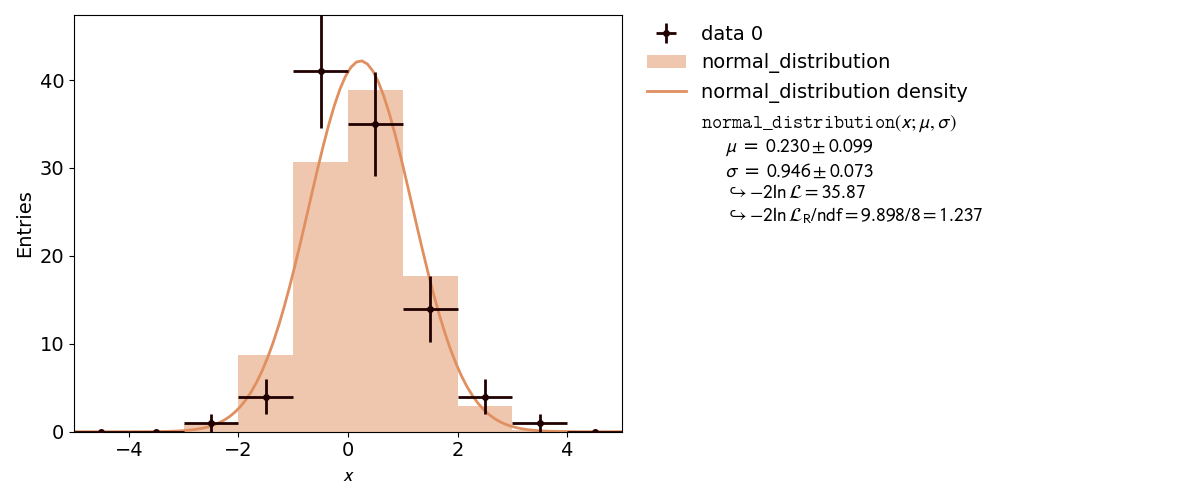
9: Histogram Fit
kafe2 is not only capable of performing XY-Fits. One way to handle one-dimensional data with kafe2 is by fitting a histogram. The distribution of a random stochastic variable follows a probability density function. The fit will determine the parameters of that density function, which the dataset is most likely to follow. To get to the height of a bin, multiply the results of the fitted function with the amount of entries N of the histogram.
kafe2go
In order to tell kafe2go that a fit is a histogram fit type: histogram has to specified
inside the YAML file.
type: histogram
n_bins: 10
bin_range: [-5, 5]
# alternatively an array for the bin edges can be specified
# bin_edges: [-5.0, -4.0, -3.0, -2.0, -1.0, 0.0, 1.0, 2.0, 3.0, 4.0, 5.0]
raw_data: [-2.7055035067034487, -2.2333305188904347, -1.7435697505734427, -1.6642777356357366,
           -1.5679848184835399, -1.3804124186290108, -1.3795713509086, -1.3574661967681951,
           -1.2985520413566647, -1.2520621390613085, -1.1278660506506273, -1.1072596181584253,
           -1.0450542861845105, -0.9892894612864382, -0.9094385163243246, -0.7867219919905643,
           -0.7852735587423539, -0.7735126880952405, -0.6845244856096362, -0.6703508433626327,
           -0.6675916809443503, -0.6566373185397965, -0.5958545249606959, -0.5845389846486857,
           -0.5835331341085711, -0.5281866305050138, -0.5200579414945709, -0.48433400194685733,
           -0.4830779584087414, -0.4810505389213239, -0.43133946043584287, -0.42594442622513157,
           -0.31654403621747557, -0.3001580802272723, -0.2517534764243999, -0.23262171181200844,
           -0.12253717030390852, -0.10096229375978451, -0.09647228959040793, -0.09569644689333284,
           -0.08737474828114752, -0.03702037295350094, -0.01793164577601821, 0.010882324251760892,
           0.02763866634172083, 0.03152268199512073, 0.08347307807870571, 0.08372272370359508,
           0.11250694814984155, 0.11309723105291797, 0.12917440700460459, 0.19490542653497123,
           0.22821618079608103, 0.2524597237143017, 0.2529456172163689, 0.35191851476845365,
           0.3648457146544489, 0.40123846238388744, 0.4100144162294351, 0.44475132818005764,
           0.48371376223538787, 0.4900044970651449, 0.5068133677441506, 0.6009580844076079,
           0.6203740420045862, 0.6221661108241587, 0.6447187743943843, 0.7332139482413045,
           0.7347787168653869, 0.7623603460722045, 0.7632360142894643, 0.7632457205433638,
           0.8088938754947214, 0.817906674531189, 0.8745869551496841, 0.9310849201186593,
           1.0060465798362423, 1.059538506895515, 1.1222643456638215, 1.1645916062658435,
           1.2108747344743727, 1.21215950663896, 1.243754543112755, 1.2521725699532695,
           1.2742444530825068, 1.2747154562887673, 1.2978477018565724, 1.304709072578339,
           1.3228758386699584, 1.3992737494003136, 1.4189560403246424, 1.4920066960096854,
           1.5729404508236828, 1.5805518556565201, 1.6857079988218313, 1.726087558454503,
           1.7511987724150104, 1.8289480135723097, 1.8602081565623672, 2.330215727183154]

model_density_function:
  model_function_formatter:
    latex_name: 'pdf'
    latex_expression_string: "\\exp{{\\frac{{1}}{{2}}(\\frac{{{x}-{mu}}}{{{sigma}}})^2}} /
    \\sqrt{{2\\pi{sigma}^2}}"
    arg_formatters:
      x: '{\tt x}'
      mu: '\mu'
      sigma: '\sigma'
  python_code: |
    def normal_distribution(x, mu, sigma):
        return np.exp(-0.5 * ((x - mu) / sigma) ** 2) / np.sqrt(2.0 * np.pi * sigma ** 2)
Python
To use a histogram fit in a Python script you can use the wrapper kafe2.hist_fit.
Alternatively you can use objects via from kafe2 import HistContainer, HistFit.
The creation of a histogram requires the user to set the limits of the histogram and the amount of bins. Alternatively the bin edges for each bin can be set manually.
import numpy as np
import kafe2


def normal_distribution(x, mu=0.01, sigma=1.0):
    return np.exp(-0.5 * ((x - mu) / sigma) ** 2) / np.sqrt(2.0 * np.pi * sigma ** 2)


# random dataset of 100 random values, following a normal distribution with mu=0 and sigma=1
data = np.random.normal(loc=0, scale=1, size=100)

# Finally, do the fit and plot it:
kafe2.hist_fit(model_function=normal_distribution, data=data, n_bins=10, bin_range=(-5, 5))
kafe2.plot()
10: Unbinned Fit
An unbinned fit is needed when there are too few data points to create a (good) histogram. If a histogram is created from too few data points information can be lost or even changed by changing the exact value of one data point to the range of a bin. With an unbinned likelihood fit it’s still possible to fit the probability density function to the data points, as the likelihood of each data point is fitted.
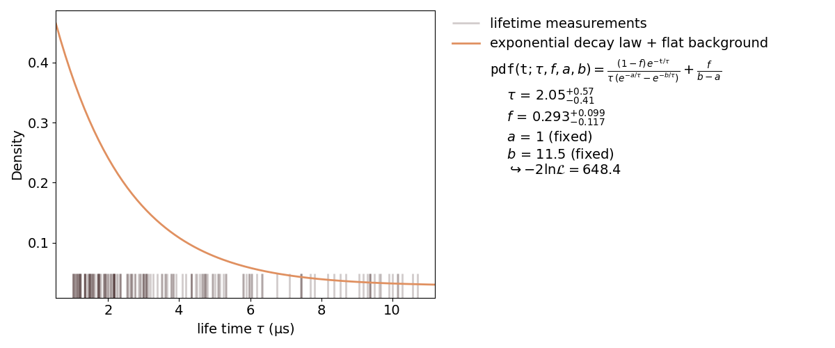
Inside a kafe2 fit, single parameters can be fixed as seen in the plot. When fixing a parameter, there must be a good reason to do so. In this case it’s the normalization of the probability distribution function. This, of course, could have been done inside the function itself. But if the user wants to change to normalization without touching the distribution function, this is a better way.
kafe2go
Similar to histogram fits, unbinned fits are defined by type: unbinned inside the YAML file.
How to fix single parameters is highlighted in the example below, as well as limiting the
background fbg to physically correct values.
type: unbinned
data: [7.420, 3.773, 5.968, 4.924, 1.468, 4.664, 1.745, 2.144, 3.836, 3.132, 1.568, 2.352, 2.132,
       9.381, 1.484, 1.181, 5.004, 3.060, 4.582, 2.076, 1.880, 1.337, 3.092, 2.265, 1.208, 2.753,
       4.457, 3.499, 8.192, 5.101, 1.572, 5.152, 4.181, 3.520, 1.344, 10.29, 1.152, 2.348, 2.228,
       2.172, 7.448, 1.108, 4.344, 2.042, 5.088, 1.020, 1.051, 1.987, 1.935, 3.773, 4.092, 1.628,
       1.688, 4.502, 4.687, 6.755, 2.560, 1.208, 2.649, 1.012, 1.730, 2.164, 1.728, 4.646, 2.916,
       1.101, 2.540, 1.020, 1.176, 4.716, 9.671, 1.692, 9.292, 10.72, 2.164, 2.084, 2.616, 1.584,
       5.236, 3.663, 3.624, 1.051, 1.544, 1.496, 1.883, 1.920, 5.968, 5.890, 2.896, 2.760, 1.475,
       2.644, 3.600, 5.324, 8.361, 3.052, 7.703, 3.830, 1.444, 1.343, 4.736, 8.700, 6.192, 5.796,
       1.400, 3.392, 7.808, 6.344, 1.884, 2.332, 1.760, 4.344, 2.988, 7.440, 5.804, 9.500, 9.904,
       3.196, 3.012, 6.056, 6.328, 9.064, 3.068, 9.352, 1.936, 1.080, 1.984, 1.792, 9.384, 10.15,
       4.756, 1.520, 3.912, 1.712, 10.57, 5.304, 2.968, 9.632, 7.116, 1.212, 8.532, 3.000, 4.792,
       2.512, 1.352, 2.168, 4.344, 1.316, 1.468, 1.152, 6.024, 3.272, 4.960, 10.16, 2.140, 2.856,
       10.01, 1.232, 2.668, 9.176]
label: "lifetime measurements"
x_label: "life time $\\tau$ (µs)"
y_label: "Density"
model_function:
  name: pdf
  latex_name: '{\tt pdf}'
  python_code: |
    def pdf(t, tau=2.2, fbg=0.1, a=1., b=9.75):
        """Probability density function for the decay time of a myon using the
        Kamiokanne-Experiment. The pdf is normed for the interval (a, b).
        :param t: decay time
        :param fbg: background
        :param tau: expected mean of the decay time
        :param a: the minimum decay time which can be measured
        :param b: the maximum decay time which can be measured
        :return: probability for decay time x"""
        pdf1 = np.exp(-t / tau) / tau / (np.exp(-a / tau) - np.exp(-b / tau))
        pdf2 = 1. / (b - a)
        return (1 - fbg) * pdf1 + fbg * pdf2
  arg_formatters:
    t: '{\tt t}'
    tau: '{\tau}'
    fbg: '{f}'
    a: '{a}'
    b: '{b}'
  latex_expression_string: "\\frac{{ (1-{fbg}) \\, e^{{ -{t}/{tau} }} }}
    {{ {tau} \\, (e^{{ -{a}/{tau} }} - e^{{ -{b}/{tau} }}) }} + \\frac{{ {fbg} }} {{ {b}-{a} }}"
model_label: "exponential decay law + flat background"
fixed_parameters:
  a: 1
  b: 11.5
limited_parameters:
  fbg: [0.0, 1.0]
Python
The fitting procedure is similar to the one of a histogram fit. How to fix single parameters is highlighted in the example below.
from kafe2.fit import UnbinnedContainer, Fit, Plot
from kafe2.fit.tools import ContoursProfiler

import numpy as np


def pdf(t, tau=2.2, fbg=0.1, a=1.0, b=9.75):
    """
    Probability density function for the decay time of a muon using the Kamiokanne-Experiment.
    The PDF is normed for the interval (a, b).

    :param t: decay time
    :param fbg: background
    :param tau: expected mean of the decay time
    :param a: the minimum decay time which can be measured
    :param b: the maximum decay time which can be measured
    :return: probability for decay time x
    """
    pdf1 = np.exp(-t / tau) / tau / (np.exp(-a / tau) - np.exp(-b / tau))
    pdf2 = 1. / (b - a)
    return (1 - fbg) * pdf1 + fbg * pdf2


# load the data from the experiment
infile = "tau_mu.dat"
dT = np.loadtxt(infile)

data = UnbinnedContainer(dT)  # create the kafe data object
data.label = 'lifetime measurements'
data.axis_labels = ['life time $\\tau$ (µs)', 'Density']

# create the fit object and set the pdf for the fit
fit = Fit(data=data, model_function=pdf)

# Fix the parameters a and b.
# Those are responsible for the normalization of the pdf for the range (a, b).
fit.fix_parameter("a", 1)
fit.fix_parameter("b", 11.5)
# constrain parameter fbg to avoid unphysical region
fit.limit_parameter("fbg", 0., 1.)

# assign latex names for the parameters for nicer display
fit.model_label = "exponential decay law + flat background"
fit.assign_parameter_latex_names(fbg='f')
# assign a latex expression for the fit function for nicer display
fit.assign_model_function_latex_expression("\\frac{{ (1-{fbg}) \\, e^{{-{t}/{tau}}} }}"
                                           "{{{tau} \\, (e^{{-{a}/{tau}}}-e^{{-{b}/{tau}}}) }}"
                                           "+ \\frac{{ {fbg}}} {{{b}-{a}}}")

fit.do_fit()  # perform the fit
fit.report(asymmetric_parameter_errors=True)  # print a fit report to the terminal

plot = Plot(fit)  # create a plot object
plot.plot(fit_info=True, asymmetric_parameter_errors=True)  # plot the data and the fit

# Optional: create a contours profile
cpf = ContoursProfiler(fit, profile_subtract_min=False)
# Optional: plot the contour matrix for tau and fbg
cpf.plot_profiles_contours_matrix(parameters=['tau', 'fbg'])

plot.show()  # show the plot(s)
11: Multifit
The premise of this example is deceptively simple: a series
of voltages is applied to a resistor and the resulting current
is measured. The aim is to fit a model to the collected data
consisting of voltage-current pairs and determine the
resistance  .
.
According to Ohm’s Law, the relation between current and voltage is linear, so a linear model can be fitted. However, Ohm’s Law only applies to an ideal resistor whose resistance does not change, and the resistance of a real resistor tends to increase as the resistor heats up. This means that, as the applied voltage gets higher, the resistance changes, giving rise to nonlinearities which are ignored by a linear model.
To get a hold on this nonlinear behavior, the model must take the temperature of the resistor into account. Thus, the temperature is also recorded for every data point. The data thus consists of triples, instead of the usual “xy” pairs, and the relationship between temperature and voltage must be modeled in addition to the one between current and voltage.
Here, the dependence  is taken to be quadratic, with
some coefficients
is taken to be quadratic, with
some coefficients  ,
,  , and
, and  :
:
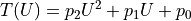
This model is based purely on empirical observations. The  dependence is more complicated, but takes the “running” of the
resistance with the temperature into account:
dependence is more complicated, but takes the “running” of the
resistance with the temperature into account:
In the above,  is the temperature in degrees Celsius,
 is an empirical “heat coefficient”, and
  is the resistance at 0 degrees Celsius, which we want to determine.
In essence, there are two models here which must be fitted to the
and data sets, and one model “incorporates”
the other in some way.
Approach 1: parameter constraints
There are several ways to achieve this with kafe2. The method chosen
here consists of two steps: First, a quadratic model is fitted to the
datasets to estimate the parameters ,
and and their covariance matrix.
Next, the model is fitted, with the temperature
being explicitly replaced by its parameterization as a function of
, and . The key here is to fit these
parameters again from the dataset, but to constrain them
to the values obtained in the previous fit.
In general, this approach yields different results than the one using a simultaneous multi-model fit, which is demonstrated in the next example.
import numpy as np

from kafe2 import XYFit, Plot


# empirical model for T(U): a parabola
def empirical_T_U_model(U, p_2=1.0, p_1=1.0, p_0=1.0):
    # use quadratic model as empirical temperature dependence T(U)
    return p_2 * U**2 + p_1 * U + p_0


# model of current-voltage dependence I(U) for a heating resistor
def I_U_model(U, R_0=1., alpha=0.004, p_2=1.0, p_1=1.0, p_0=1.0):
    # use quadratic model as empirical temperature dependence T(U)
    _temperature = empirical_T_U_model(U, p_2, p_1, p_0)
    # plug the temperature into the model
    return U / (R_0 * (1.0 + _temperature * alpha))


# -- Next, read the data from an external file

# load all data into numpy arrays
U, I, T = np.loadtxt('OhmsLawExperiment.dat', unpack=True)  # data
sigU, sigI, sigT = 0.2, 0.1, 0.5  # uncertainties

T0 = 273.15  # 0 degrees C as absolute Temperature (in Kelvin)
T -= T0  # Measurements are in Kelvin, convert to °C

# -- Finally, go through the fitting procedure

# Step 1: perform an "auxiliary" fit to the T(U) data
auxiliary_fit = XYFit(
    xy_data=[U, T],
    model_function=empirical_T_U_model
)
auxiliary_fit.data_container.axis_labels = ("Voltage (V)", "Temperature (°C)")
auxiliary_fit.data_container.label = "Temperature data"
auxiliary_fit.model_label = "Parametrization"

# (Optional): Assign names for models and parameters
auxiliary_fit.assign_model_function_expression('{1}*{U}^2 + {2}*{U} + {3}')
auxiliary_fit.assign_model_function_latex_expression(r'{1}\,{U}^2 + {2}\,{U} + {3}')

# declare errors on U
auxiliary_fit.add_error(axis='x', err_val=sigU)

# declare errors on T
auxiliary_fit.add_error(axis='y', err_val=sigT)

# perform the auxiliary fit
auxiliary_fit.do_fit()

# (Optional) print the results
auxiliary_fit.report(asymmetric_parameter_errors=True)

# (Optional) plot the results
auxiliary_plot = Plot(auxiliary_fit)
auxiliary_plot.plot(asymmetric_parameter_errors=True)

# Step 2: perform the main fit
main_fit = XYFit(
    xy_data=[U, I],
    model_function=I_U_model
)

# declare errors on U
main_fit.add_error(axis='x', err_val=sigU)
# declare errors on I
main_fit.add_error(axis='y', err_val=sigI)

# constrain the parameters
main_fit.add_matrix_parameter_constraint(
    names=auxiliary_fit.parameter_names,
    values=auxiliary_fit.parameter_values,
    matrix=auxiliary_fit.parameter_cov_mat,
    matrix_type='cov'  # default matrix type is cov, this kwarg is just for clarity
)
main_fit.data_container.axis_labels = ("Voltage (V)", "Current (A)")
main_fit.data_container.label = "Current data"
main_fit.model_label = "Temperature-dependent conductance"

# (Optional): Assign names for models and parameters
main_fit.assign_parameter_latex_names(alpha=r'\alpha_\mathrm{T}')
main_fit.assign_model_function_expression('{U} / ({0} * (1 + ({2}*{U}^2 + {3}*{U} + {4}) * {1}))')
main_fit.assign_model_function_latex_expression(r'\frac{{{U}}}{{{0} \cdot (1 + ({2}{U}^2 + {3}{U} + {4}) \cdot {1})}}')

# Step 4: do the fit
main_fit.do_fit()

# (Optional) print the results
main_fit.report(asymmetric_parameter_errors=True)

# (Optional) plot the results
plot = Plot(main_fit)
plot.plot(asymmetric_parameter_errors=True)

plot.show()
Approach 2: multi-model fit
There are several ways to achieve this with kafe2. The method chosen
here is to use the Multifit functionality
to fit both models simultaneously to the and
datasets.
In general, this approach yields different results than the one using
parameter constraints, which is demonstrated in the example called
fit_with_parameter_constraints.
import numpy as np

from kafe2 import XYFit, MultiFit, Plot


# empirical model for T(U): a parabola
def empirical_T_U_model(U, p_2=1.0, p_1=1.0, p_0=1.0):
    # use quadratic model as empirical temperature dependence T(U)
    return p_2 * U**2 + p_1 * U + p_0

# model of current-voltage dependence I(U) for a heating resistor
def I_U_model(U, R_0=1., alpha=0.004, p_2=1.0, p_1=1.0, p_0=1.0):
    # use quadratic model as empirical temperature dependence T(U)
    _temperature = empirical_T_U_model(U, p_2, p_1, p_0)
    # plug the temperature into the model
    return U / (R_0 * (1.0 + _temperature * alpha))


# -- Next, read the data from an external file

# load all data into numpy arrays
U, I, T = np.loadtxt('OhmsLawExperiment.dat', unpack=True)  # data
sigU, sigI, sigT = 0.2, 0.1, 0.5  # uncertainties

T0 = 273.15  # 0 degrees C as absolute Temperature (in Kelvin)
T -= T0  # Measurements are in Kelvin, convert to °C

# -- Finally, go through the fitting procedure

# Step 1: construct the singular fit objects
fit_1 = XYFit(
    xy_data=[U, T],
    model_function="empirical_T_U_model: U p_2=1.0 p_1=1.0 p_0=1.0 -> p_2 * U^2 + p_1 * U + p_0"
)
fit_1.add_error(axis='y', err_val=sigT)  # declare errors on T
fit_1.data_container.axis_labels = ("Voltage (V)", "Temperature (°C)")
fit_1.data_container.label = "Temperature data"
fit_1.model_label = "Parametrization"

fit_2 = XYFit(
    xy_data=[U, I],
    model_function="I_U_model: U R_0 alpha=4e-3 p_2 p_1 p_0 -> U / (R_0 * (1 + alpha * (p_2 * U^2 + p_1 * U + p_0)))"
)
fit_2.add_error(axis='y', err_val=sigI)  # declare errors on I
fit_2.data_container.axis_labels = ("Voltage (V)", "Current (A)")
fit_2.data_container.label = "Current data"
fit_2.model_label = "Temperature-dependent conductance"

# Step 2: construct a MultiFit object
multi_fit = MultiFit(fit_list=[fit_1, fit_2], minimizer='iminuit')
#multi_fit.set_parameter_values(alpha=0.004)

# Step 3: Add a shared error error for the x axis.
multi_fit.add_error(axis='x', err_val=sigU, fits='all')

# (Optional): assign names for models and parameters
multi_fit.assign_parameter_latex_names(alpha=r'\alpha_\mathrm{T}')

# Step 4: do the fit
multi_fit.do_fit()

# (Optional): print the results
multi_fit.report(asymmetric_parameter_errors=True)

# (Optional): plot the results
plot = Plot(multi_fit, separate_figures=True)
plot.plot(asymmetric_parameter_errors=True)

plot.save()  # Automatically saves the plots to different files.

plot.show()