User Guide
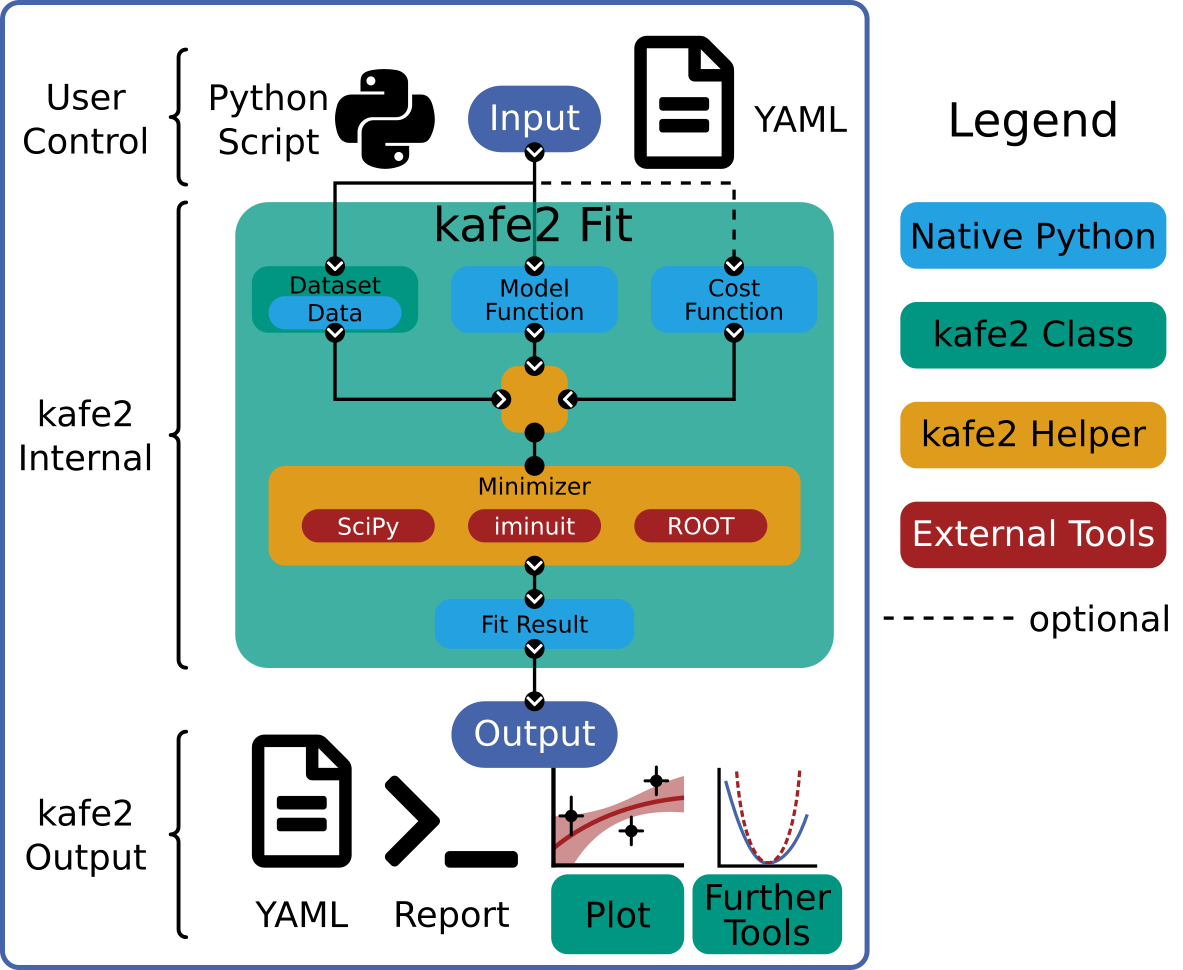
For performing fits with kafe2, the user need to specify the data, model function and
optionally a cost function to be optimized. Mathematical details are explained
in section Mathematical Foundations.
In most cases the cost function defaults to a negative-log-likelihood
function or, in simple cases or if explicitely requested, the least-squares method.
This information is passed to a FitBase-derived object.
More information can be found in the Fitting-section below.
Then there are multiple ways of displaying and using the fit results. They can either be used directly inside a Python-script, printed to the terminal, or plotted. For further analysis, the Contours Profiler is a very helpful tool to display parameter correlations.
Data handling
Data Container
In kafe2, your data is organized using data containers, which come in different types to suit various data formats.
XY Container
If your data consists of paired x and y values, use an XYContainer:
from kafe2 import XYContainer
xy_data = XYContainer(x_data=[1.0, 2.0, 3.0, 4.0], y_data=[2.3, 4.2, 7.5, 9.4])
Unbinned and Indexed Container
For one-dimensional data, kafe2 offers IndexedContainer and UnbinnedContainer:
from kafe2 import IndexedContainer, UnbinnedContainer
idx_data = IndexedContainer([5.3, 5.2, 4.7, 4.8])
unbinned_data = UnbinnedContainer([5.3, 5.2, 4.7, 4.8])
Histogram Container
If you have histogram data, use a HistContainer.
You can either specify bin edges or let kafe2 create equidistant bins for you:
from kafe2 import HistContainer
# Creating a HistContainer with equidistant bins
histogram = HistContainer(n_bins=10, bin_range=(-5, 5))

# Creating a HistContainer with specified bin edges
histogram = HistContainer(bin_edges=[-5.0, -4.0, -3.0, -2.0, -1.0, 0.0, 1.0, 2.0, 3.0, 4.0, 5.0])
After creating the histogram, it can be filled with data points.
This can be done directly when creating the container with the fill_data keyword or
afterwards with the fill method.
Data points lying outside the bin range will be stored in an underflow or overflow bin and are
not considered when performing the fit.
from kafe2 import HistContainer
histogram = HistContainer(n_bins=10, bin_range=(-5, 5),
                          fill_data=[-7.5, 1.23, 5.74, 1.9, -0.2, 3.1, -2.75, ...])
# Alternative way
histogram = HistContainer(n_bins=10, bin_range=(-5, 5))
histogram.fill([-7.5, 1.23, 5.74, 1.9, -0.2, 3.1, -2.75, ...])
Instead of filling the histogram with raw data, the bin height can be set manually with
set_bins.
When doing so, rebinning and other options won’t be available.
from kafe2 import HistContainer
histogram = HistContainer(n_bins=5, bin_range=(0, 5))
histogram.set_bins([1, 3, 5, 2, 0], underflow=2, overflow=0)
Data Labels
Label your data and specify axis labels to keep important metadata and make your finral plots invormative:
The name of the dataset or its label is set with the label property.
Axis labels can be set with the x_label and
y_label properties or the
axis_labels property:
from kafe2 import XYContainer
# Creating an XYContainer object
xy_data = XYContainer(x_data=[1.0, 2.0, 3.0, 4.0], y_data=[2.3, 4.2, 7.5, 9.4])
# Setting labels
xy_data.label = 'My Data'
xy_data.axis_labels = ['Time $\\tau$ (µs)', 'My $y$-label']
Setting Labels is available for all container types.
Uncertainties
Specifying uncertainties is crucial for obtaining meaningful fit results. Uncertainties can be independent or correlated.
Independent uncertainties
To add independent uncertainties to your data, use the add_error method:
from kafe2 import XYContainer
# Creating an XYContainer object
data = XYContainer(x_data=[1.0, 2.0, 3.0, 4.0], y_data=[2.3, 4.2, 7.5, 9.4])
data.add_error(axis='x', err_val=0.3)  # +/-0.3 for all data points in x-direction
data.add_error(axis='y', err_val=0.15, relative=True)  # +/-15% for all points in y-direction
The axis keyword is is only used with XYContainers for the add_error
method.
If err_val is a single float the same uncertainty is applied to all data points.
If err_val is a list of floats with the same length as the corresponding data,
each entry in err_val is applied to the data point with the same index.
Fitting
Creating the correct FitBase derived object can simply be done with the
Fit function, which automatically determines the correct fit type for a
DataContainerBase derived object:
from kafe2 import XYContainer, Fit
xy_data = XYContainer(x_data=[1.0, 2.0, 3.0, 4.0],
                      y_data=[2.3, 4.2, 7.5, 9.4])
# Create an XYFit object from the xy data container.
# By default, a linear function f=a*x+b will be used as the model function.
line_fit = Fit(data=xy_data)
# further additions like constraints go here
line_fit.do_fit()
Alternatively XYFit, HistFit, UnbinnedFit or
IndexedFit can be used to create fits with corresponding datasets.
Warning
Always run the do_fit function of the Fit object when everything is set.
Only when calling this function the fit will be performed.
Setting a model function
kafe2 fit objects accept normal Python functions as model functions.
The first parameter of those functions will be used as the independent parameter
(the parameter on the x axis of plots).
The default parameter values of the Python function will be used as starting values for the fit,
unless overwritten with the set_parameter_values method.
def linear_model(x, a, b):
    # Our first model is a simple linear function
    return a * x + b

def exponential_model(x, A0=1., x0=5.):
    # Our second model is a simple exponential function
    # The kwargs in the function header specify parameter defaults.
    return A0 * np.exp(x/x0)

xy_data = XYContainer(x_data=[1.0, 2.0, 3.0, 4.0],
                      y_data=[2.3, 4.2, 7.5, 9.4])

# Create 2 Fit objects with the same data but with different model functions
linear_fit = Fit(data=xy_data, model_function=linear_model)
exponential_fit = Fit(data=xy_data, model_function=exponential_model)
The display names for the model function and its parameters can be changed like this:
linear_fit.assign_model_function_name("line")
linear_fit.assign_parameter_names(a='A', b='b', x='t')
linear_fit.assign_model_function_expression("{a}{x} + {b}")
exponential_fit.assign_model_function_latex_name("\\exp")
exponential_fit.assign_parameter_latex_names(A0='A_0', x0='x_0', x='\\tau')
exponential_fit.assign_model_function_latex_expression("{A0} e^{{{x}/{x0}}}")
The latex parameter names and expressions define the graphical output when plotting while the non latex methods define the output names when reporting the fit results to the terminal.
Note
Special characters inside the strings need to be escaped. E.g. a single \ needs to be
\\.
Note
Inside the latex expression string, { and } for latex expressions like \\frac
need to be doubled, because single curly brackets are used for replacing the parameters with
their respective latex names.
E.g. kafe2 tries to replace {x0} with its latex string x_0 in this example.
Parameter Constraints
When performing a fit, some values of the model function might have already been determined in previous experiments. Those results and uncertainties can then be used to constrain the given parameters in a new fit. This eliminates the need to manually propagate the uncertainties on the final fit results, as it’s now done numerically.
Simple parameter constraints are set with the add_parameter_constraint method:
# Constrain model parameters to measurements
fit.add_parameter_constraint(name='l',   value=l,   uncertainty=delta_l)
fit.add_parameter_constraint(name='r',   value=r,   uncertainty=delta_r)
fit.add_parameter_constraint(name='y_0', value=y_0, uncertainty=delta_y_0, relative=True)
Note
The names have to be identical to the argument names in the model function. The parameter
names can be accessed with the fit parameter_names property.
If the uncertainties of several parameter constraints are correlated the
add_matrix_parameter_constraint method can be used instead.
Please refer to the API Documentation for more information.
Fixing and limiting parameters
Limiting the parameters of a model function can be useful for improving the convergence of a fit by reducing the size of the parameter space in which it searches for the global cost function minimum. This is commonly done when the fit result of one or more parameters is expected to fall in a certain range or when the model function is not valid for some parameter values (e.g. a negative amplitude). For fits with many parameters fixing some of them at first and fitting multiple times might also help.
Fixing parameters is done with the fix_parameter method and limiting with the
limit_parameter method. Releasing a fixed parameter is performed with
release_parameter and unlimiting a parameter with
unlimit_parameter:
fit.fix_parameter("a", 1)
fit.fix_parameter("b", 11.5)
fit.release_parameter("a")
# limit parameter fbg to avoid unphysical region
fit.limit_parameter("fbg", 0., 1.)
fit.unlimit_parameter("fbg")
Note
The names have to be identical to the argument names in the model function. The parameter
names can be accessed with the fit parameter_names property.
Fixed parameters can be released with the release_parameter method and
limited parameters can be unlimited with the unlimit_parameter method.
Minimizers
Currently the use of three different minimizers is supported. By default iminuit is
used. If iminuit is not available, kafe2 falls back to
scipy.optimize.minimize.
The usage of a specific minimizer can be set during initialization of any
FitBase-object with the minimizer keyword.
Depending on the installed minimizers this can either be 'iminuit', 'scipy' or
'root'.
Additional keywords for the instantiation can be passed as a dict via the
minimizer_kwargs keyword when creating a fit object derived from FitBase.
Logging
To enable the output of the minimizer, set up a logger before calling do_fit:
import logging
logger = logging.getLogger()
logger.setLevel(logging.INFO)
This currently only works for the scipy and iminuit minimizer.
For more detailed information increase the logging level to logging.DEBUG.
This will give a more verbose output when using iminuit.
The logger level should be reset to logging.WARNING before plotting.
Otherwise matplotlib will create logging messages as well.
Access the fit results
The do_fit method returns a dictionary containing most of the relevant
results. Additionally the results can be printed to the terminal with report.
The parameter values can also be accessed via the parameter_values property
as well as the symmetric and asymmetric parameter uncertainties and the correlation and
covariance matrices via their respective properties:
fit = Fit(my_dataset)  # create a fit object
# perform the fit and calculate asymmetric uncertaintes
result = fit.do_fit(asymmetric_parameter_errors=True)
fit.report()  # print fit results to the terminal
par_vals = fit.parameter_values
par_errs = fit.parameter_errors
par_errs_asym = fit.asymmetric_parameter_errors
par_ocv_mat = fit.parameter_cov_mat
par_cor_mat = fit.parameter_cor_mat
A typical dictionary returned by the do_fit method looks like this:
{'did_fit': True,
 'cost': 1.7759115950075888,
 'ndf': 2,
 'goodness_of_fit': 1.7759115950075888,
 'cost/ndf': 0.8879557975037944,
 'chi2_probability': 0.41149607486886164,
 'parameter_values': OrderedDict([('a', 2.468773761415478), ('b', -0.3219331193129483)]),
 'parameter_cov_mat': array([[ 0.0443453 , -0.1108627 ],
                             [-0.1108627 ,  0.33239252]]),
 'parameter_errors': OrderedDict([('a', 0.2105624096609012), ('b', 0.576478065203752)]),
 'parameter_cor_mat': array([[ 1.       , -0.9131448],
                             [-0.9131448,  1.       ]]),
 'asymmetric_parameter_errors': None}
Plotting
For visualizing the results of a fit, kafe2 provides a Plot class, backed by
matplotlib.pyplot.figure objects.
This means that all customizations possible with Matplotlib can be applied to kafe2 plots as well.
The Plot class supports the simultaneous plotting of multiple fits, which, by default, appear in the same figure. To plot each fit on a separate figure, set separate_figures=True:
import matplotlib.pyplot as plt
from kafe2 import Plot

# Plotting multiple fits on the same figure
p = Plot([fit_1, fit_2])

# For separate figures use:
# p = Plot([fit_1, fit_2], separate_figures=True)

# Customize the plot here
p.plot()
plt.show()
Running the plot function performs the actual plot.
Note that there are some customizations already possible by setting the corresponding
keyword arguments for the plot function.
After plotting, the according matplotlib objects can be
accessed via the figures and axes properties.
The Plot class also supports the use of data containers, for only plotting data points.
Customization
Note
Ensure that the plot method is called after all customizations are done,
as some changes may not appear in the plot otherwise.
Axis Range
Set the plot range using the x_range and y_range
properties:
# set the same range for all plots
p.x_range = (0, 10)
p.y_range = (-5, 25)

# set different ranges for each plot
p.x_range = [(0, 10), (-5, 5)]
p.y_range = [(-5, 25), (10, 100)]

p.plot()  # plot method must come after the customization
Axis Scale
Change the axis scale to logarithmic using the x_scale and
y_scale properties:
# set the same scale for all fits in this plot object
p.x_scale = "log"
p.y_scale = "linear

# Change the scale for each fit individually
# Only use this when `separate_figures=True` is set in the Plot constructor
p.x_scale = ["linear", "log"]
p.y_scale = ["log", "log"]

p.plot()  # plot method must come after the customization
Axis Labels
By default, uses labels specified for each dataset (see Data Labels). Overwrite axis labels for each fit with:
# Set the same axis labels for all fits in this plot object
p.x_label = "My $x$-label"
p.y_label = "Voltage [mV]"

# Set different labels for each fit
p.x_label = ["$x_1$", "My other label for $x_2$"]
p.y_label = ["$Y_1$", "$y_2$"]

p.plot()  # plot method must come after customization
Plot Style
Customize each graphic element individually.
Available plot_types for XYFits are
'data', 'model_line', 'model_error_band', 'ratio', 'ratio_error_band' and ‘model’ which
is hidden by default.
The plot_types may differ for different types of fits.
The currently set keywords can be obtained with the get_keywords method.
With customize new values can be added or existing values can
be modified. Using '__del__' will delete the keyword and '__default__' will reset
it.
Hide specific elements from the plot (e.g. the uncertainty band):
# The array length must match the number of fits handled by this plot
p.customize('model_error_band', 'hide', [True])
Change the name for the data set and suppress the second output:
p.customize('data', 'label', [(0, "test data"), (1, '__del__')])
Customize marker type, size and color for the marker and error bars:
p.customize('data', 'marker', [(0, 'o'), (1,'o')])
p.customize('data', 'markersize', [(0, 5), (1, 5)])
p.customize('data', 'color', [(0, 'blue'), (1,'blue')]) # note: although 2nd label is suppressed
p.customize('data', 'ecolor', [(0, 'blue'), (1, 'blue')]) # note: although 2nd label is suppressed
Customize the model function:
p.customize('model_line', 'color', [(0, 'orange'), (1, 'lightgreen')])
p.customize('model_error_band', 'label', [(0, r'$\pm 1 \sigma$'), (1, r'$\pm 1 \sigma$')])
p.customize('model_error_band', 'color', [(0, 'orange'), (1, 'lightgreen')])
Additionally customization using matplotlib functions:
import matplotlib as mpl
mpl.rc('axes', labelsize=20, titlesize=25)
Contours Profiler
The class ContoursProfiler provides methods for profiling the cost function in one or two parameters. These are used to extract confidence intervals for the fit parameters or two-dimensional confidence contours for pairs of parameters.
First, a ContoursProfiler object must be created from a Fit object:
from kafe2 import ContoursProfiler
cpf = ContoursProfiler(fit)
By default, the one and two  contours are calculated. Other values can be
specified in the ContoursProfiler constructor:
contours are calculated. Other values can be
specified in the ContoursProfiler constructor:
from kafe2 import ContoursProfiler
cpf = ContoursProfiler(fit, contour_sigma_values=(1, 2, 3))
Often confidence levels are not reported in units of , but in percentages
(e.g. 95%). To specify e.g. the 90% and 95% confidence level contours:
from kafe2 import ContoursProfiler
cpf = ContoursProfiler(fit, contour_cl_values=(0.9, 0.95))
Note that only one of contour_cl_values and contour_sigma_values can be specified at the same time. In most cases a graphical representation is desired. Call the method plot_profiles_contours_matrix() to show profile likelihood and confidence curves for all parameters in a matrix arrangement:
cpf.plot_profiles_contours_matrix() # plot the contour profile matrix for all parameters
It is also possible to show the profile likelihood of a single parameter:
cpf.plot_profile('<paramer name>')
or to display only selected confidence contours:
plot_contours('<name1>', '<name2>')
Consult the api documentation on details how to restrict the displayed ranges or for special plot options. For cases where further investigations are needed, functions exist to return the results as numpy arrays:
xp, cost_function = cpf. get_profile('<paramer name>', low=lower_bound, high=upper_bound)
or to show selected confidence contours:
vals1, vals2 = get_contours('<name1>', 'n<ame2>')
Todo
Add more detail, examples already use the contours profiler.