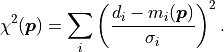
Mathematical Foundations
This chapter describes the mathematical foundations on which kafe2 is built, in particular the method of maximum likelihood and how confidence intervals are determined from the profile likelihood.
When performing a fit (as a physicist) the problem is as follows: you have some amount of measurement data from an experiment that you need to compare to one or more models to figure out which of the models - if any - provides the most accurate description of physical reality. You typically also want to know the values of the parameters of a model and the degree of (un)certainty on those values.
For very simple problems you can figure this out analytically: you take a formula and simply plug in your measurements. However, as your problems become more complex this approach becomes much more difficult - or even straight up impossible. For this reason complex problems are typically solved numerically: you use an algorithm to calculate a result that only approximates the analytical solution but in a way that is much easier to solve. kafe2 is a tool for the latter approach.
Cost Functions
In the context of parameter estimation, a model  (where
  is just some index) is a function of the parameters
  .
During the fitting process the parameters are varied in such a way that the
agreement between the model and the corresponding data
.
During the fitting process the parameters are varied in such a way that the
agreement between the model and the corresponding data  becomes “best”.
This of course means that we need to somehow define “good” or “bad” agreement - we need a metric.
This metric is called a loss function or cost function.
It is defined in such a way that a lower cost function value corresponds with a “better” agreement
between a model and our data.
becomes “best”.
This of course means that we need to somehow define “good” or “bad” agreement - we need a metric.
This metric is called a loss function or cost function.
It is defined in such a way that a lower cost function value corresponds with a “better” agreement
between a model and our data.
The cost functions implemented by kafe2 are based on the method of maximum likelihood.
The idea behind this method is to maximize the likelihood function  which represents the probability with which a model
 would result in the data
  that we ended up measuring:
where  describes the probability of measuring the data
point given the corresponding model prediction
describes the probability of measuring the data
point given the corresponding model prediction  .
This approach allows for a statistical interpretation of our fit results as we will see later.
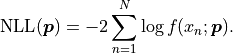
Instead of the likelihood described above however, we are instead using twice its negative
logarithm, the so-called negative log-likelihood (NLL):
.
This approach allows for a statistical interpretation of our fit results as we will see later.
Instead of the likelihood described above however, we are instead using twice its negative
logarithm, the so-called negative log-likelihood (NLL):

This transformation is allowed because logarithms are
strictly monotonically increasing functions, and therefore the negative logarithm of any
function will have its global minimum at the same place where the original function is maximal.
The model  that minimizes the NLL
will therefore also maximize the likelihood.
that minimizes the NLL
will therefore also maximize the likelihood.
While the above transformation may seem nonsensical at first, there are important advantages to calculating the negative log-likelihood over the likelihood:
The product of the probabilities
 is replaced by a
sum over the logarithms of the probabilities
is replaced by a
sum over the logarithms of the probabilities  .
In the context of a computer program sums are preferable over products because they can be
calculated more quickly and because a product of many small numbers can lead to
arithmetic underflow.
.
In the context of a computer program sums are preferable over products because they can be
calculated more quickly and because a product of many small numbers can lead to
arithmetic underflow.Because the probabilities
oftentimes contain exponential functions,
calculating their logarithm is actually faster because it reduces the number of necessary
operations.Algorithms for numerical optimization minimize functions so they can be directly used to optimize the NLL.
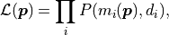
As an example, let us consider the likelihood function of data that follows a
normal distribution around means  with standard deviations (uncertainties)
  :
:
![\mathcal{L}
= \prod_i P(\mu_i, \sigma_i, d_i)
= \prod_i \frac{1}{\sqrt[]{2 \pi} \: \sigma_i}
\exp \left[ - \frac{1}{2} \left( \frac{d_i - \mu_i}{\sigma_i} \right)^2 \right].](../_images/math/ee4d1135b2a8ca937e96117a86a8922ed4bffdf7.png)
The immediate trouble that we run into with this definition is that we have no idea what the
means are - after all these are the “true values” that our data deviates from.
However, since we are trying to determine the likelihood with which our data would be produced
given our model we can set  .
.
Note
Conceptually uncertainties are typically associated with the data even though
they represent deviations from the model .
However, because the normal distribution is symmetric this does not have an effect on the
likelihood function  (as long as the uncertainties
  do not depend on the model
).
do not depend on the model
).
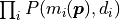
For the NLL we now find:
![\mathrm{NLL}(\bm{p})
= -2 \log \mathcal{L}({\bm p}) \\
= - 2 \log \prod_i \frac{1}{\sqrt[]{2 \pi} \: \sigma_i}
\exp \left[ - \frac{1}{2} \left( \frac{d_i - m_i({\bm p})}{\sigma_i} \right)^2 \right] \\
= - 2 \sum_i \log \frac{1}{\sqrt[]{2 \pi} \: \sigma_i}
+ \sum_i \left( \frac{d_i - m_i({\bm p})}{\sigma_i} \right)^2 \\
=: - 2 \log L_\mathrm{max} + \chi^2({\bm p}) .](../_images/math/64198e2d2cff8f14a01a7b269089c7b6c423b622.png)
As we can see the logarithm cancels out the exponential function of the normal
distribution and we are left with two parts:
The first is a part represented by  that only depends on the
uncertainties but not on the model or the data .
This is the minimum value the NLL could possibly take on if the model
were to exactly fit the data .
The second part can be summed up as
that only depends on the
uncertainties but not on the model or the data .
This is the minimum value the NLL could possibly take on if the model
were to exactly fit the data .
The second part can be summed up as
As mentioned before, this is much easier and faster to calculate than the original
likelihood function.
If the uncertainties are constant we can ignore the first part and directly use
 (chi-squared) as our cost function because
we are only interested in differences between cost function values.
This special case of the method of maximum likelihood is known as the method of least squares
and it is by far the most common cost function used for fits.
(chi-squared) as our cost function because
we are only interested in differences between cost function values.
This special case of the method of maximum likelihood is known as the method of least squares
and it is by far the most common cost function used for fits.
Covariance
The cost function that we discussed in the previous section assumes
that our data points are subject to uncertainties .
With this notation we implicitly assumed that our uncertainties are independent of one another:
that there is no relationship between the uncertainties of any two individual data points.
Independent uncertainties are frequently caused by random fluctuations in the measurement values,
either because of technical limitations of the experimental setup (electronic noise, mechanical
vibrations) or because of the intrinsic statistical nature of the measured observable (as is typical
in quantum mechanics, e. g. radioactive decays).
However, there are also correlated uncertainties that arise due to effects that distort multiple measurements in the same way. Such uncertainties can for example be caused by a random imperfection of the measurement device which affects all measurements equally. The uncertainties of the measurements taken with such a device are no longer uncorrelated, but instead have one common uncertainty.
Historically uncertainties have been divided into statistical and systematic uncertainties.
While this is appropriate when propagating the uncertainties of the input variables by hand it is
not a suitable distinction for a numerical fit.
In kafe2 multiple uncertainties are combined to construct a so-called covariance matrix.
This is a matrix with the pointwise data variances  on its diagonal and the covariances
  between two data points outside the diagonal.
By using this covariance matrix for our fit we can estimate the uncertainty of our model parameters
numerically with no need for propagating uncertainties by hand.
between two data points outside the diagonal.
By using this covariance matrix for our fit we can estimate the uncertainty of our model parameters
numerically with no need for propagating uncertainties by hand.
As mentioned before, the diagonal elements of our covariance matrix represent the variances
 of our data points.
They simply represent the uncertainty of a single data point while ignoring all other
data points.
An element outside the diagonal at position
of our data points.
They simply represent the uncertainty of a single data point while ignoring all other
data points.
An element outside the diagonal at position  represents the covariance
between points and
represents the covariance
between points and  :
:
![\mathrm{Cov}_{ij}
= E[ (d_i - E[d_i])(d_j - E[d_j]) ]
= E[d_i \cdot d_j] - E[d_i] \cdot E[d_j],](../_images/math/5b8116a0dbdcceb08478db7635ab7e3bec12131a.png)
where  is the expected value of a variable.
The covariance is a measure of the joint variability of and
- but for a meaningful interpretation it needs to be considered relative to the
pointwise uncertainties .
We therefore define the so-called Pearson correlation coefficient
is the expected value of a variable.
The covariance is a measure of the joint variability of and
- but for a meaningful interpretation it needs to be considered relative to the
pointwise uncertainties .
We therefore define the so-called Pearson correlation coefficient  as follows:

The correlation is normalized to the interval ![[-1, 1]](../_images/math/92b4b754966e4a581f924d4bfd1b0db7ab47c886.png) .
Its absolute value is a measure of how strongly the residuals
.
Its absolute value is a measure of how strongly the residuals  depend on one another.
In other words, the absolute value of measures how much information
you get about
depend on one another.
In other words, the absolute value of measures how much information
you get about  or
or  if you know the other one.
For
if you know the other one.
For  they are completely independent from one another.
For
they are completely independent from one another.
For  and are directly proportional to one
another with a positive (negative) proportional constant for
and are directly proportional to one
another with a positive (negative) proportional constant for
 (
( ).
Let’s look at some toy samples for different values of :
).
Let’s look at some toy samples for different values of :
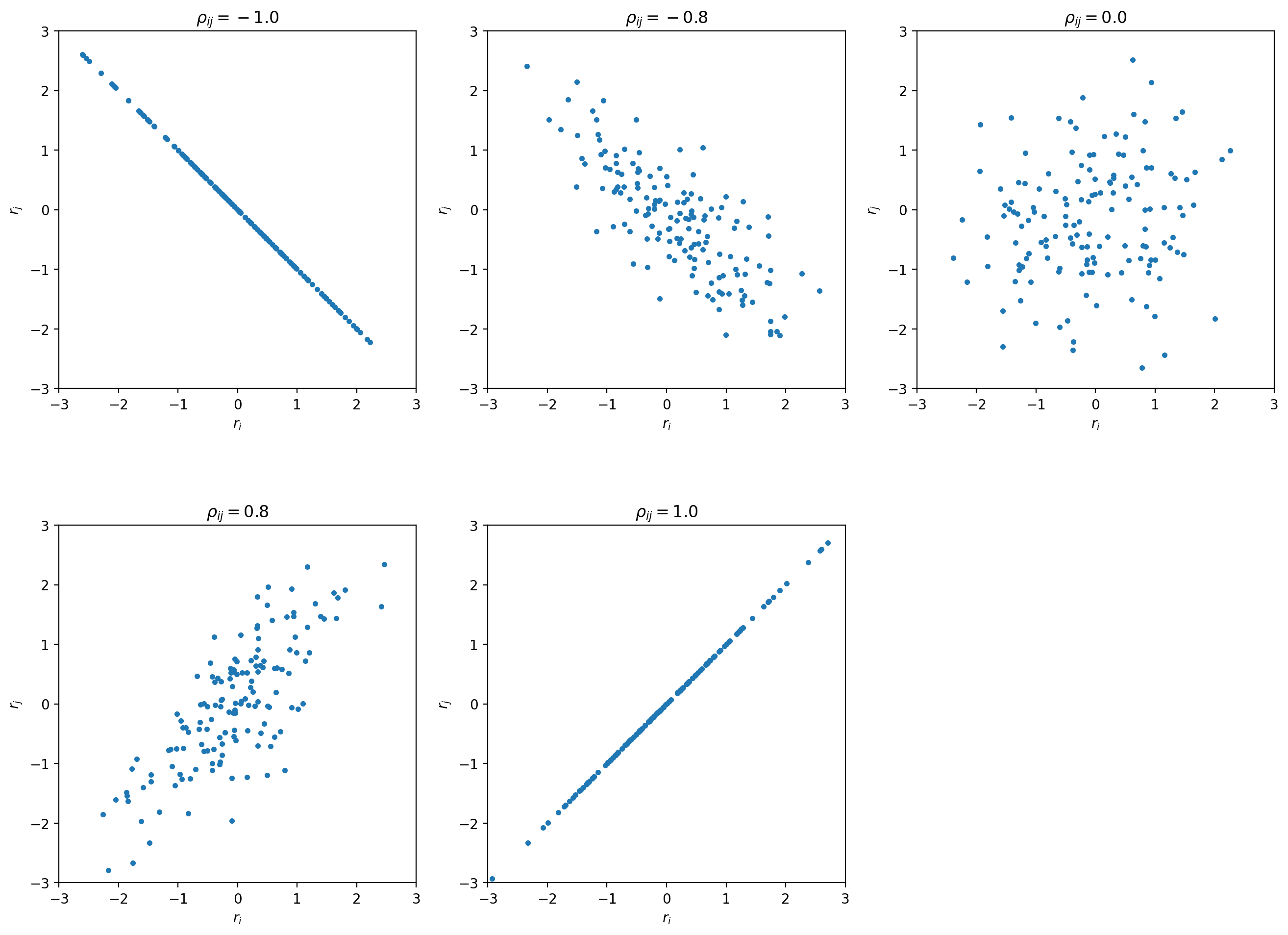
For  the sample forms a circle around (0,0).
As the absolute value of increases the sample changes its shape to a tilted
ellipse - some combinations of and become more likely than others.
For
the sample forms a circle around (0,0).
As the absolute value of increases the sample changes its shape to a tilted
ellipse - some combinations of and become more likely than others.
For  the ellipse becomes a line -
in this degenerate case we really only have one source of uncertainty that affects two data points.
the ellipse becomes a line -
in this degenerate case we really only have one source of uncertainty that affects two data points.
Covariance Matrix Construction
In a physics experiment it is typically necessary to consider more than one source of uncertainty.
Let us consider the following example:
we want to measure Earth’s gravitational constant  by dropping things from various heights
and timing the time they take to hit the ground with a stopwatch.
We assume an independent uncertainty of
by dropping things from various heights
and timing the time they take to hit the ground with a stopwatch.
We assume an independent uncertainty of  for each data point
because humans are not able to precisely align pressing the button of a stopwatch with the actual
event.
For one reason or another the stopwatch we’re using is also consistently
off by a few percentage points.
To account for this we assume a fully correlated (
for each data point
because humans are not able to precisely align pressing the button of a stopwatch with the actual
event.
For one reason or another the stopwatch we’re using is also consistently
off by a few percentage points.
To account for this we assume a fully correlated ( ) uncertainty of
 for all data points.
To determine the variance of a single data point we can simply add up the variances
of the uncertainty sources:
for all data points.
To determine the variance of a single data point we can simply add up the variances
of the uncertainty sources:

As it turns out we can use the same approach for the covariances: we can simply add up the covariance matrices of the different uncertainty sources to calculate a total covariance matrix:

The next question would then be how you would determine the covariance matrices for the
individual uncertainty sources.
A useful approach is to split a covariance matrix into a vector of uncertainty  and the corresponding correlation matrix
  :
:
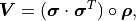
where  is the Hadamard product (a.k.a. Schur product).
In other words, the components of
is the Hadamard product (a.k.a. Schur product).
In other words, the components of  are calculated by simply multiplying the
components of
are calculated by simply multiplying the
components of  and at
the same position.
If we assume that we have three data points we can express the human uncertainty as follows:
and at
the same position.
If we assume that we have three data points we can express the human uncertainty as follows:
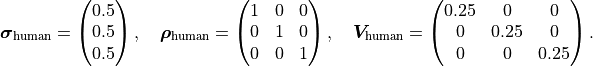
Because the human uncertainties of the individual data points are completely independent from one
another the covariance/correlation matrix is a diagonal matrix.
On the other hand, given some data points
the watch uncertainty is expressed like this:

Because the watch uncertainties of the individual data points are fully correlated all components of the correlation matrix are equal to 1. However, this does not necessarily mean that all components of the covariance matrix are also equal. In this example the watch uncertainty per data point is relative, meaning that the absolute uncertainty differs from data point to data point.
If we were to visualize the correlations of the uncertainty components described above, we would find that samples of the human component form a circle while samples from the watch component form a line. If we were to visualize the total uncertainty we would end up with the mixed case where the sample forms an ellipse.
Correlated Least Squares
We previously defined the  cost function like this:
This definition is only correct if the uncertainties for each data point are independent.
If we want to consider the correlations between uncertainties we need to use
the covariance matrix  instead of the pointwise uncertainties :

Notably the division by the uncertainties has been replaced by a matrix inversion.
This is because the uncorrelated definition is a special case of the correlated definition.
If the uncertainties are completely uncorrelated then is a diagonal matrix.
To invert such a matrix you only need to replace the diagonal elements
 with
with  .
.
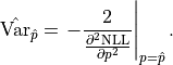
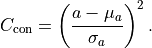
Parameter Confidence Intervals
When we perform a fit we are not only interested in the parameter values that fit our data “best”,
we also want to determine the uncertainty on our result.
The standard method with which fitting tools determine parameter confidence intervals is to make
use of the so-called Rao-Cramér-Fréchet bound.
It states for the variance of the estimator of a single parameter estimate  :
:
![\mathrm{Var}_{\hat{p}} \ge 2 \frac{1 + \frac{\partial b}{\partial p}}
{E \left[ \frac{\partial^2 \mathrm{NLL}}{\partial p^2} \right]},](../_images/math/15648e9d1e71019ed37fe5896b8a5decbc72a325.png)
where  is the bias of the estimator.
Because the bias cannot be easily computed it is usually assumed to be 0 in practice
(check with a Monte Carlo study when in doubt).
Furthermore, because likelihood methods are efficient (if an efficient estimator exists at all)
the uncertainties on the fit results decrease “quickly” as more data is added and the RCF bound
becomes an equality.
Finally, in the large sample limit (i.e. if you have “enough” data and your uncertainties are
sufficiently small) the expectation in the
denominator can be replaced with the derivative of the likelihood at the cost function minimum.
All together we thus find for the uncertainty of our fit result:
is the bias of the estimator.
Because the bias cannot be easily computed it is usually assumed to be 0 in practice
(check with a Monte Carlo study when in doubt).
Furthermore, because likelihood methods are efficient (if an efficient estimator exists at all)
the uncertainties on the fit results decrease “quickly” as more data is added and the RCF bound
becomes an equality.
Finally, in the large sample limit (i.e. if you have “enough” data and your uncertainties are
sufficiently small) the expectation in the
denominator can be replaced with the derivative of the likelihood at the cost function minimum.
All together we thus find for the uncertainty of our fit result:
The default output of a fitting tool are as the parameter value and
 as the parameter error.
For reasons that will become clear in the following sections these errors will also be referred to
as the “parabolic errors”.
If the estimator of a parameter is normally distributed then so-called
confidence intervals can be calculated which (for a random dataset) contain the true value
as the parameter error.
For reasons that will become clear in the following sections these errors will also be referred to
as the “parabolic errors”.
If the estimator of a parameter is normally distributed then so-called
confidence intervals can be calculated which (for a random dataset) contain the true value
 with a given probability called the confidence level
  .
For a confidence interval
.
For a confidence interval  the confidence level is calculated by integrating the
probability density function of the normal distribution:
the confidence level is calculated by integrating the
probability density function of the normal distribution:
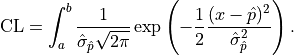
The confidence interval bounds are frequently chosen symmetrically around and
expressed as multiples of  .
For example, the “
.
For example, the “ interval”
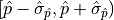 has a confidence level
of approximately 68%.
has a confidence level
of approximately 68%.
If is normally distributed then the method described above can be used directly.
In the large sample limit this is always the case for maximum likelihood estimators.
If you don’t have enough data (or if you don’t know) you will need to use e.g. the method described
in the next section.
Profile Likelihood (1 Parameter)
Let’s assume we have a fit with only a single parameter  .
If the estimator
.
If the estimator  is normally distributed then the negative log-likelihood
 is a parabola.
If is varied by
is a parabola.
If is varied by  standard deviations
  from the
optimal value in either direction then increases by
from the
optimal value in either direction then increases by  .
For a non-Gaussian estimator the confidence intervals derived from the RCF bound can be approximated
by determining the parameter values at which
.
For a non-Gaussian estimator the confidence intervals derived from the RCF bound can be approximated
by determining the parameter values at which
 is equal to the squared
equivalent sigma value .
In general the confidence intervals determined in this manner with this “profile likelihood method”
will be asymmetrical.
In loose terms, if the cost function value increases very sharply when we move away from the cost
function minimum then this tells us that even a small deviation from our fit result would result in
a significantly worse fit, making large deviations unlikely.
Conversely, if the cost function value increases very slowly when we move away
from the cost function minimum then this tells us that a deviation from our
fit result would result in a fit that is only slightly worse than our optimal fit result,
making such a deviation from our fit result quite possible.
is equal to the squared
equivalent sigma value .
In general the confidence intervals determined in this manner with this “profile likelihood method”
will be asymmetrical.
In loose terms, if the cost function value increases very sharply when we move away from the cost
function minimum then this tells us that even a small deviation from our fit result would result in
a significantly worse fit, making large deviations unlikely.
Conversely, if the cost function value increases very slowly when we move away
from the cost function minimum then this tells us that a deviation from our
fit result would result in a fit that is only slightly worse than our optimal fit result,
making such a deviation from our fit result quite possible.
The obvious problem with the profile likelihood method described above is that in practice fits
will almost always have more than one parameter
(the additional parameters being denoted as ).
So how do we determine the values for these other parameters as we vary just one of them?
The solution is to choose in such a
way that  becomes minimal.
In practical terms this means that we fix to several values near the cost function minimum
and then perform a fit over all other parameters for each of these values
(this process is called profiling).
In this context the parameters are called nuisance parameters:
we don’t care about their values (right now) but we need to include them in our fits for
a statistically correct result.
becomes minimal.
In practical terms this means that we fix to several values near the cost function minimum
and then perform a fit over all other parameters for each of these values
(this process is called profiling).
In this context the parameters are called nuisance parameters:
we don’t care about their values (right now) but we need to include them in our fits for
a statistically correct result.
If the estimator is normally distributed then the confidence intervals derived from
the profile likelihood are the same as the ones derived from the RCF bound - if you suspect that
this is not the case you should always check the profiles of the parameters.
The easiest way to do this is to set the flag profile = True when calling kafe2.xy_fit or
kafe2.plot.
The parabolic parameter uncertainties are then replaced with the edges of the
1- -intervals determined from the profile likelihood.
Because these intervals are not necessarily symmetric around the cost function minimum they are
referred to as asymmetric parameter errors in kafe2
(in Minuit they are called Minos errors).
-intervals determined from the profile likelihood.
Because these intervals are not necessarily symmetric around the cost function minimum they are
referred to as asymmetric parameter errors in kafe2
(in Minuit they are called Minos errors).
When the above flag is set kafe2 will then also create plots of the profile likelihood in
addition to the regular plots.
As an example, let us look at the profile of the parameter
from the double slit example:
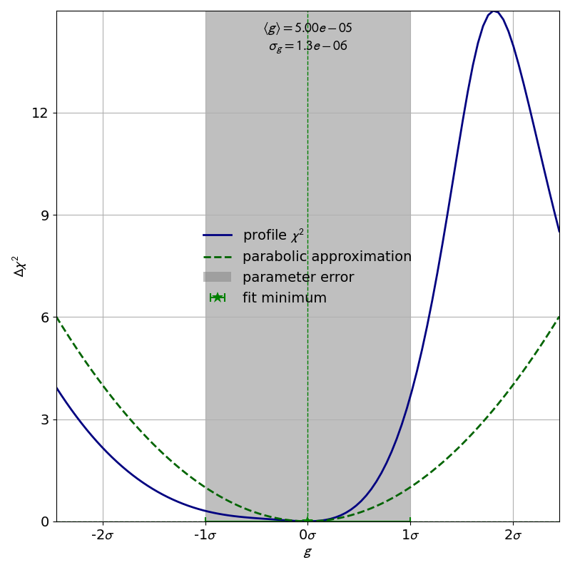
The profile of this parameter is very clearly asymmetric and not even close to the parabolic approximation of a normal distribution. If we had only looked at the parabolic parameter error we could have unknowingly assumed confidence intervals that are very inaccurate.
Profile Likelihood (2 parameters)
In the previous section we learned about the profiles of single fit parameters which serve as a replacement for the parabolic errors of single fit parameters. In this section we will learn about so-called contours, which serve as a replacement for the covariance of two fit parameters. Conceptually profiles and contours are very similar. A profile can be used to define confidence intervals for a single parameter with a certain probability of containing the true value of a parameter while a contour defines a confidence region with a certain probability of containing a pair of parameters. Let us start by looking at the contours produced in the double slit example:
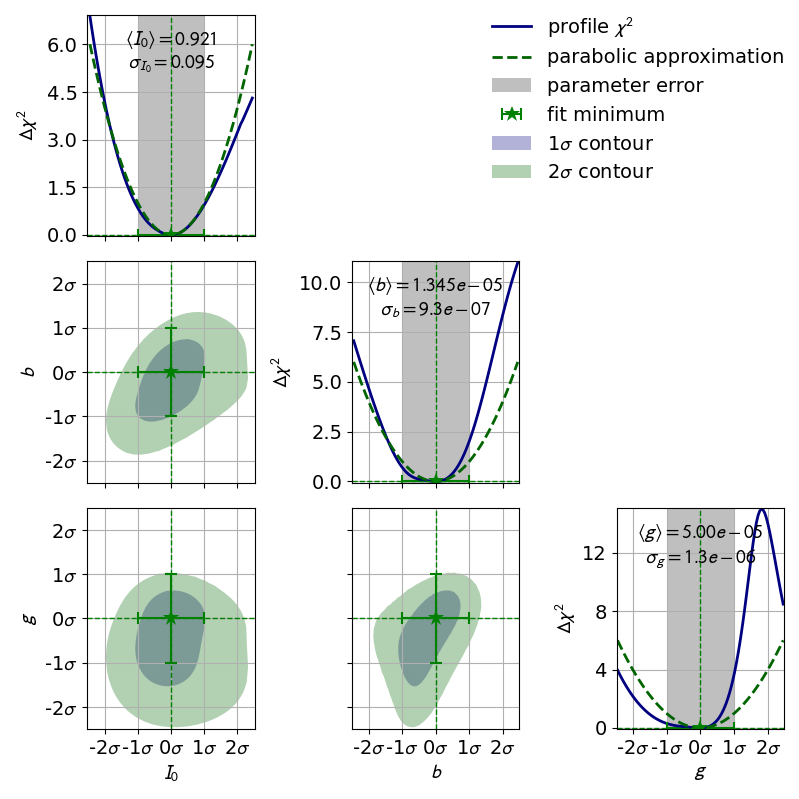
In this visualization the confidence region inside the contours is colored.
By looking at the legend we find that the contours correspond to
1 and 2 .
Notably the confidence levels of the corresponding confidence regions are not
the same as in one dimension.
In one dimension 1 corresponds to roughly 68% while
2 corresponds to roughly 95%.
We could derive these confidence levels by integrating the probability density function
of the standard normal distribution over the interval ![[-\sigma , \sigma]](../_images/math/56622cf23958e5f5950007cb52d6c6940b56c7ab.png) for a desired value.
In two dimensions we instead integrate the PDF of the uncorrelated standard bivariate
normal distribution over a circle with radius around the origin:
for a desired value.
In two dimensions we instead integrate the PDF of the uncorrelated standard bivariate
normal distribution over a circle with radius around the origin:
![\mathrm{CL}(\sigma)
= \int_0^\sigma dr \int_0^{2 \pi} d \varphi \ r \frac{1}{2 \pi} e^{- \frac{r^2}{2}}
= \int_0^\sigma dr \ r e^{- \frac{r^2}{2}}
= \left[ -e^{-\frac{r^2}{2}} \right]_0^\sigma
= 1 - e^{-\frac{\sigma^2}{2}}.](../_images/math/248f0c48b45b23ae885bc570c1b2d69b88190daa.png)
With this formula we now find
 .
.
Note
So far there has been no mention of how a contour for a given
 could be calculated.
This is because (efficiently) calculating these contours is not straightforward and
even in kafe2 this is an area of active development.
could be calculated.
This is because (efficiently) calculating these contours is not straightforward and
even in kafe2 this is an area of active development.
The parabolic equivalent of a contour is to look at the parameter covariance matrix and to extrapolate the correlated distribution of two estimators. As with the input uncertainties the confidence region calculated this way will always be an ellipse. For (nearly) normally distributed estimators such as the estimators from the exponential fit in the “model functions” example the calculated contours will then look something like this:
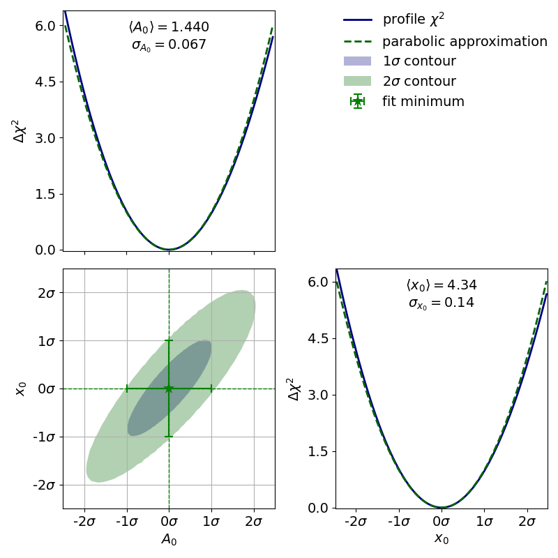
If the estimators were normally distributed the 1--contour would reach exactly from
 to
to  while the 2--contour would reach exactly from
  to
to  .
As we can see the deviation from this is very small so we can probably use the parameter covariance
matrix (or the parabolic parameter errors and the parameter correlation matrix) without issue.
If we require highly precise confidence intervals for our parameters
this might not be acceptable though.
.
As we can see the deviation from this is very small so we can probably use the parameter covariance
matrix (or the parabolic parameter errors and the parameter correlation matrix) without issue.
If we require highly precise confidence intervals for our parameters
this might not be acceptable though.
Note
The degree to which confidence intervals/regions are distorted from their parabolic approximation depends on the scale at which the profile likelihood is calculated. Because every function minimum can be accurately approximated by a parabola at infinitesimally small scales (Taylor expansion) the parabolic approximation becomes more accurate for small parameter uncertainties. Conversely, for large parameter uncertainties the parabolic approximation of the profile likelihood becomes less accurate.
Nonlinear Models
In the previous section we discussed the profile likelihood and how it can be used to calculate confidence intervals for our fit parameters. We also discussed how it is necessary to use this method if the parameter estimators are not normally distributed. What was not discussed is how to determine if an estimator is normally distributed in the first place. This is where this section comes in.
Linear Models
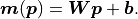
Let us assume we have some vector of data points with corresponding
constant Gaussian uncertainties (that can also be correlated).
A linear model is then defined as a model
that is a multilinear function of its  parameters
  :
:
where the weights  and biases
  are simply real numbers (the biases
here have nothing to do with the bias in the RCF bound).
Put another way, each model value
are simply real numbers (the biases
here have nothing to do with the bias in the RCF bound).
Put another way, each model value  is a linear combination of the
parameter values plus some bias .
We can express the same relationship as above with a weight matrix
is a linear combination of the
parameter values plus some bias .
We can express the same relationship as above with a weight matrix  and a bias vector
  :
:
If we now use the method of least squares ( ) to estimate the
optimal fit parameters  we get a very useful property:
the estimators of our parameters are normally distributed.
We can therefore skip the (relatively) expensive process of profiling the parameters!
we get a very useful property:
the estimators of our parameters are normally distributed.
We can therefore skip the (relatively) expensive process of profiling the parameters!
Let us look at some examples for linear models in the context of xy fits since
those are the most common.
Let us therefore assume that we have some y data measured at
x values 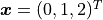 .
For our model function we choose the first degree polynomial
.
For our model function we choose the first degree polynomial 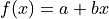 .
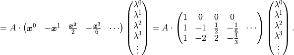
We can thus express our model like this:
.
We can thus express our model like this:
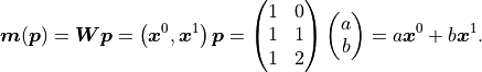
The upper indices of vectors are to be interpreted as powers of said vectors using the
Hadamard/Schur product (component-wise multiplication).
In the above equation we only have a weight matrix 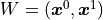 but no bias vector.
We can clearly see that the first degree polynomial (a line) is a linear model.
Let’s take a look at the third degree polynomial
but no bias vector.
We can clearly see that the first degree polynomial (a line) is a linear model.
Let’s take a look at the third degree polynomial  :
:
Again we find that the model is a linear function
of its parameters .
A third degree polynomial is therefore also a linear model.
This is even though the model function is not a linear function
of the independent variable  .
However, this was never required in our definition of linear models to begin with because
is not one of our fit parameters.
In fact, all polynomials are linear models.
.
However, this was never required in our definition of linear models to begin with because
is not one of our fit parameters.
In fact, all polynomials are linear models.
Nonlinear Models
Now that we have defined linear models, the definition of nonlinear models is
rather easy: a model that is not a linear model.
The natural consequence of this is that the estimators of our fit parameters are no longer
guaranteed to be normally distributed.
We will therefore need to resort to calculating confidence intervals from the profile likelihood.
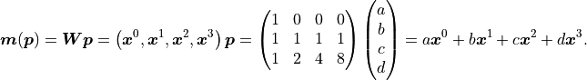
Let us consider an exponential model as an example: 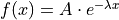 .
It is simply not possible to express this function using only a finite weight matrix
and a bias vector .
We would instead need an infinitely large matrix and infinitely many parameters.
With the same x vector as before we find:
.
It is simply not possible to express this function using only a finite weight matrix
and a bias vector .
We would instead need an infinitely large matrix and infinitely many parameters.
With the same x vector as before we find:
Note
We could of course just cut off the series at some point to approximate the exponential function.
This would be equivalent to approximating the exponential function with a polynomial.
But this would not allow us to calculate an estimate for the parameter  - which is
very often the entire point of a physics experiment.
- which is
very often the entire point of a physics experiment.
Unfortunately, even with a linear model function the regression problem as a whole can become
nonlinear if certain kafe2 features are used.
As of right now these features are uncertainties in x direction for xy fits
and uncertainties relative to the model.
This is because when using those features the uncertainties that we feed to our
negative log-likelihood are no longer constant.
Instead they become a function of the fit parameters:  .
.
Another complication is that we then have to consider the full Gaussian likelihood rather
than just to avoid biasing our results:
![\mathrm{NLL}(\bm{p})
= - 2 \log L_\mathrm{max}(\bm p) + \chi^2({\bm p})
= - 2 \sum_i \log \frac{1}{\sqrt[]{2 \pi} \: \sigma_i(\bm{p})} + \chi^2(\bm{p}) \\
= N \log (2 \pi) + 2 \sum_i^N \log \sigma_i(\bm{p}) + \chi^2(\bm{p})
=: N \log (2 \pi) + C_\mathrm{det}(\bm{p}) + \chi^2(\bm{p}).](../_images/math/ea2349f36b7e87a49d97fc812593eee1d3a942e9.png)
As with our derivation of we end up with a constant term  which we can ignore because we are only interested in the differences in cost.
We also get a new term
which we can ignore because we are only interested in the differences in cost.
We also get a new term 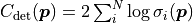 that
we need to consider when our uncertainties depend on our fit parameters.
The new term results in higher cost when the uncertainties increase.
If we didn’t add
that
we need to consider when our uncertainties depend on our fit parameters.
The new term results in higher cost when the uncertainties increase.
If we didn’t add  while handling parameter-dependent uncertainties
we would end up with a bias towards parameter values for which the uncertainties are increased
because those values result in a lower value for .
The subscript “det” is short for determinant, the reason for which should become clear when we
look at the full Gaussian likelihood with correlated uncertainties represented
by a covariance matrix
while handling parameter-dependent uncertainties
we would end up with a bias towards parameter values for which the uncertainties are increased
because those values result in a lower value for .
The subscript “det” is short for determinant, the reason for which should become clear when we
look at the full Gaussian likelihood with correlated uncertainties represented
by a covariance matrix  :
:
![\mathrm{NLL}(\bm{p})
= - 2 \log L_\mathrm{max}(\bm{p}) + \chi^2(\bm{p})
= - 2 \log \left[ (2 \pi)^{-\frac{N}{2}}
\frac{1}{\sqrt{\det \bm{V}(\bm{p})}} \right] + \chi^2(\bm{p}) \\
= N \log (2 \pi) + \log \det \bm{V}(\bm{p}) + \chi^2(\bm{p})
=: N \log (2 \pi) + C_\mathrm{det}(\bm{p}) + \chi^2(\bm{p})](../_images/math/39c82fa8c80b082c63d041e4ac0df7b42fbd5510.png)
The constant term is the same as with the uncorrelated uncertainties but term we’re interested in
has changed to 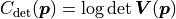 .
If the uncertainties are uncorrelated then the covariance matrix is diagonal
and the result is equal to the term we found earlier.
.
If the uncertainties are uncorrelated then the covariance matrix is diagonal
and the result is equal to the term we found earlier.
Note
Handling correlated uncertainties that are a function of our fit parameters
is computationally expensive because this means that we need to recalculate
the inverse (actually Cholesky decomposition) of our covariance many times which has
complexity  for data points - on modern hardware
this is typically not an issue though.
for data points - on modern hardware
this is typically not an issue though.
Uncertainties In x Direction
Now that we know how to handle parameter-dependent uncertainties we can use this knowledge
to handle a very common problem:
fitting a model with model function  to data with x values
  and
uncertainties in both the x and the y direction.
The uncertainties in the y direction
and
uncertainties in both the x and the y direction.
The uncertainties in the y direction  can be used directly.
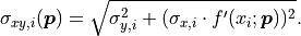
For the x uncertainties
can be used directly.
For the x uncertainties  we need a trick:
we project the uncertainties onto the y axis by
multiplying them with the corresponding model function derivative by x
we need a trick:
we project the uncertainties onto the y axis by
multiplying them with the corresponding model function derivative by x  :
:
The formula for the pointwise projected xy uncertainties  can
be generalized for the equivalent covariance matrices
can
be generalized for the equivalent covariance matrices  and
and  :
:

where is again the Hadamard product (a.k.a. Schur product) where two matrices
are multiplied on a component-by-component basis.
We are also implicitly assuming that  is a vectorized function à la
NumPy that returns a vector of derivatives for a vector of x values
is a vectorized function à la
NumPy that returns a vector of derivatives for a vector of x values  .
.
Uncertainties Relative To The Model
Relative uncertainties are very common.
For example, the uncertainties of digital multimeters are
typically specified as a percentage of the reading.
Unfortunately such uncertainties are therefore relative to the true values which we don’t know.
The standard approach for handling relative uncertainties is therefore to specify them relative
to the data points which we do know.
However, this approach introduces a bias:
if the random fluctuation represented by an uncertainty causes our data to have
a reduced (increased) absolute value
then the relative uncertainties are underestimated (overestimated).
This causes a bias towards models with smaller absolute values in our fit because we are giving
data points that randomly happen to have a low absolute value a higher weight than data points
with a high absolute value -
and this bias increases for large relative uncertainties.
A better result can be achieved by specifying uncertainties relative to the model
rather than the data .
Because the model (ideally) converges against the true values in the large sample limit we no longer
give a higher weight to data that randomly happens to have a lower absolute value.
The price we pay for this is that our total uncertainty becomes a function of our model parameters
which results in an increase in computation time as described above.
Gaussian Approximation Of The Poisson Distribution
kafe2 has a built-in approximation of the Poisson distribution where the Gaussian uncertainty is assumed as:
The rationale for using the square root of the model rather than the square
root of the data
is the same as with the relative uncertainties described in the previous section.
The benefit of using this approximation of the Poisson distribution instead of the
Poisson distribution itself is that it is capable of
handling additional Gaussian uncertainties on our data.
Hypothesis Testing
So far we have used cost functions to compare how good or bad certain models
and parameter values fit our data relative to each other -
but we have never discussed how good or bad a fit is in an absolute sense.
Luckily for us there is a metric that we can use:
 , where is simply the sum of the
squared residuals that we already know and
, where is simply the sum of the
squared residuals that we already know and  is the
number of degrees of freedom that our fit has.
The basic definition of is that it’s simply the number
of data points
is the
number of degrees of freedom that our fit has.
The basic definition of is that it’s simply the number
of data points  minus the number of parameters
  :
:
Conceptually the number of degrees of freedom are the number of “extra measurements”
over the minimum number of data points needed to fully specify a model with
linearly independent parameters.
If our model is not fully specified then our cost function has multiple
(or even infinitely many) global minima.
For example, a line with model function  has two
linearly independent parameters and as such needs at least two data points to be fully
specified.
has two
linearly independent parameters and as such needs at least two data points to be fully
specified.
If our model accurately describes our data, and if our assumptions about
the uncertainties of our data are correct, then
has an expected value of 1.
If is smaller (larger) than 1 we might be
overestimating (underestimating) the uncertainties on our data.
If is much larger than 1 then our model may not
accurately describe our data at all.
To further quantify these rather loose criteria we can make use of Pearson’s chi-squared test.
This is a statistical test that allows us to calculate the probability
 with which we can expect to observe deviations from
our model that are at least as large as the deviations that we saw in our data.
To conduct this test we first need to define the so-called
with which we can expect to observe deviations from
our model that are at least as large as the deviations that we saw in our data.
To conduct this test we first need to define the so-called  distribution.
This distribution has a single parameter
distribution.
This distribution has a single parameter  and when sampling from this distribution,
the samples from standard normal distributions
and when sampling from this distribution,
the samples from standard normal distributions  are simply squared and then added up:
The deviations of our data relative to its true values (represented by our model) and
normalized to its uncertainties follow such standard normal distributions.
We can therefore expect the sum of the squares of these deviations  to follow
a
to follow
a  distribution with
  -
if our model and our assumptions about the uncertainties of our data are correct.
We can associate the following cumulative distribution function (CDF)
-
if our model and our assumptions about the uncertainties of our data are correct.
We can associate the following cumulative distribution function (CDF)
 with the distribution:
To calculate the probability with which we would expect a
value larger than what we got for our fit
(i.e. the probability of our fit being worse if we were to repeat it with a new random dataset)
we can now simply use:

In kafe2 is also referred to as the probability.
We can use this number to determine if deviations from our
assumed model are statistically significant.
The concept of as can be generalized for non-Gaussian likelihoods
where the metric becomes goodness of fit
per degree of freedom  .
For a negative log likelihood
.
For a negative log likelihood  with model and
data it is defined like this:
with model and
data it is defined like this:
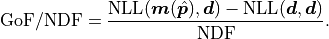
We are subtracting the so-called saturated likelihood  (the minimum value our NLL could have if our model were to perfectly describe our data)
from the global cost function minimum
(the minimum value our NLL could have if our model were to perfectly describe our data)
from the global cost function minimum  and then divide this difference by .
As before the expected value of is 1
if our model and our assumptions about the uncertainties of our data are correct.
and then divide this difference by .
As before the expected value of is 1
if our model and our assumptions about the uncertainties of our data are correct.
Calculating Data Uncertainties from
Many fitting tools allow users to fit a model to data without specifying any data uncertainties.
This seems to be at odds with our current understanding of Gaussian likelihood-based fits where
we always required our data to have some amount of uncertainty.
So how does this work?
The “solution” is to first give all data points an uncorrelated uncertainty of 1 and to scale
these uncertainties after the fit in such a way that is equal to 1.
This approach has a big problem which makes it unsuitable for physics experiments:
we cannot do any hypothesis tests because we are
implicitly assuming that our model is 100% correct.
This goes against the very purpose of many physics experiments where experimenters are trying to
determine if a theoretical model is consistent with experimental data.
For example, at the Large Hadron Collider the standard model of particle physics has undergone very thorough testing that continues to this day. So far, no statistically significant deviations from the standard model have been found - which is actually a bummer for theoretical physicists. You see, we know for a fact that the standard model is incomplete because (among other things) it does not include gravity. If we were to find an area in which the predictions of the standard model are incompatible with the measured data this would give theorists an important clue for a new theory that could potentially fix the problems of the standard model.
Fixing And Constraining Parameters
kafe2 allows users to fix fit parameters.
The practical consequence of this is that one of our fit parameters becomes a constant and
is not changed during the fit.
Because this effectively lowers the number of fit parameters we have to consider the number
of fixed parameters  in the calculation of the number of degrees of fredom:

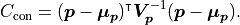
It’s also possible to constrain fit parameters.
Constraints are effectively direct measurements of our fit parameters and they
increase the cost of our fit if they are not exactly met.
For example, the additional cost  of a Gaussian constraint for
fit parameter with mean
of a Gaussian constraint for
fit parameter with mean  and standard deviation
  can be calculated like this:
We can of course generalize this concept to account for correlations between
parameters as defined by a covariance matrix  :
:
If we define any constraints we are adding more data to our fit.
We therefore also have to increase
by the number of constraints  :
:

A simple parameter constraint that constrains a single parameter counts as one constraint.
On the other hand, a matrix parameter constraint that constrains  parameters at once
counts as constraints.
parameters at once
counts as constraints.
Data/Fit Types
A large percentage of fits can be expressed as an XYFit.
However, there are cases where an XYFit is not suitable;
kafe2 offers alternatives fit types for those cases.
Typically these alternative fit types are associated with alternative data (container) types
so both concepts are explained simultaneously in this section.
For example, an XYFit uses an XYContainer to hold its xy data
while a HistFit uses a HistContainer to hold and bin its data.
For the following considerations always describes the vector of fit parameters.
Unless mentioned otherwise fits calculate their cost from a data vector
and a model vector  .
.
XYFit
Let’s start with the most common fit type: XYFit.
The data associated with this fit type consists of two vectors of equal length:
a vector of x data and a vector of y data .
Our model values are calculated as  ,
they are a function of our x data and our fit parameters.
As the difference in notation implies the x and y axes are not treated in the same way.
The x axis is interpreted as the independent variable of our fit while the y data values
and y model values
,
they are a function of our x data and our fit parameters.
As the difference in notation implies the x and y axes are not treated in the same way.
The x axis is interpreted as the independent variable of our fit while the y data values
and y model values  are what we ultimately
compare to calculate the negative log-likelihood.
are what we ultimately
compare to calculate the negative log-likelihood.
Note
Although we only have a few discreet x values for which we have to calculate our model
 , our model function
is still expected to be a continuous function of .
, our model function
is still expected to be a continuous function of .
A visualization of XYFit is fairly straightforward:
the xy axes of our fix directly correspond to the axes of a plot.
IndexedFit
Conceptually IndexedFit is a simplified version of XYFit:
we only have a data vector and no independent variable at all.
Instead we calculate the model vector
as a function of just the fit parameters.
In kafe2 IndexedFit is visualized by interpreting the indices of the data/model
vectors as x values and the corresponding xth entry of those vectors as the y value.
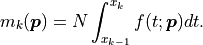
HistFit
HistFit handles one-dimensional data points by binning them
according to some bin edges  to form our data vector
 .
By default the model function that is fitted to these bins is a
probability density function for the observed values .
The bin heights predicted by our model are obtained by integrating
over a given bin and multiplying the result with :
.
By default the model function that is fitted to these bins is a
probability density function for the observed values .
The bin heights predicted by our model are obtained by integrating
over a given bin and multiplying the result with :
The amplitude of our distribution is therefore not one of the fit parameters;
we are effectively fitting a density function to a normalized histogram.
By setting density=False when creating the HistFit object an arbitrary model can
be fit to a histogram that is not normalized.
Unlike with XYFit or IndexedFit the default distribution assumed for the
data of a HistFit is the Poisson distribution rather than the normal distribution.
UnbinnedFit
Just like HistFit an UnbinnedFit accepts a vector of
one-dimensional data points in conjunction with a probability density function
for these values as its model function.
As the name implies the data is not binned.
Instead, because our model function can be interpreted as a probability density we can simply
calculate the negative log-likelihood like this:
In kafe2 UnbinnedFit is visualized by interpreting the independent variable as the
x axis of a plot and the height of the probability density function as the y axis.
Additionally, a thin, vertical line is added for each data point to indicate
the density of our data.
CustomFit
Unlike the other fit types discussed so far, CustomFit does not explicitly use data
or a model .
Instead the user has to manually define how the cost function value is calculated from the fit
parameters .
Because any potential data is outside kafe2 there is no built-in visualization (plotting)
available except for the fit parameter profiles/contours calculated by ContoursProfiler.
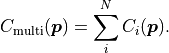
MultiFit
A MultiFit is constructed from regular fits with cost functions
 .
The idea behind
.
The idea behind MultiFit is rather simple:
multiple models that share at least one parameter are
simultaneously fitted to their respective data.
In accordance with the method of maximum likelihood the optimal fit parameters are those that make
the observed combination of individual datasets the most likely.
The corresponding cost function can simply be calculated as:
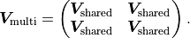
If a MultiFit is built from several fits that assume Gaussian uncertainties,
it’s possible to specify uncertainties that are correlated between those fits.
For example, in the case of two fits that have a fully correlated source of uncertainty expressed
by a covariance matrix  the effective covariance matrix
 for the
 MultiFit becomes:
Cost Functions
So far we almost universally assumed that the uncertainties of our data can be described with a normal distribution. However, this is not always the case. For example, the number of radioactive decays in a given time interval follows a Poisson distribution. In kafe2 such distinctions are handled via the cost function, the function that in one way or another calculates a scalar cost from the data, model, and uncertainties of a fit. This section describes the built-in cost functions that kafe2 provides.
Cost Function
The by far most common cost function used is the cost function that assumes a normal
distribution for the uncertainties of our data.
In kafe2 the name is strictly speaking a misnomer because the actual cost calculation considers
the full likelihood rather than just in order to handle non-constant uncertainties.
For data points with corresponding model values
and uncorrelated (but possible non-constant) uncertainties  the cost function value is calculated like this:
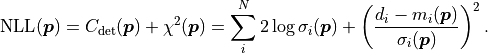
If the uncertainties are instead correlated as described by a covariance matrix
the cost function value becomes:

Poisson Cost Function
The Poisson cost function assumes - as the name implies - a Poisson distribution for our data.
Compared to the normal distribution the Poisson distribution has two important features:
Firstly the data values (but not the model values )
have to be positive integers, and secondly the mean and variance are inherently linked.
We can define the likelihood function  of the Poisson distribution like this:
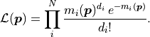
The negative log-likelihood  thus becomes:
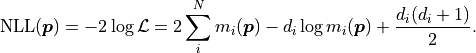
Notably depends only on the data and the model
but not on any specified uncertainties .
The advantage is that we don’t need to specify any uncertainties -
but the significant disadvantage is that we can’t specify any uncertainties either.
In such cases the cost function in the following section will need to be used.
Gauss Approximation Cost Function
Because a Poisson distribution cannot handle Gaussian data uncertainties the Poisson distribution
is frequently approximated with a normal distribution.
The easiest approach is to simply derive the uncertainties
from the data :

However, as described in the previous section about linear models,
this leads to a bias towards small model values .
In kafe2 the uncertainties are therefore derived from the model values:
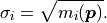
Just like before these uncertainties can be easily combined with other sources of uncertainty
by simply adding up the (co)variances.
However, this approach has an important limitation:
it is only valid if the model values are large enough
(something like  ).
This is because for small model values the asymmetry of the Poisson distribution and the portion
of the normal distribution that resides in the unphysical region with
).
This is because for small model values the asymmetry of the Poisson distribution and the portion
of the normal distribution that resides in the unphysical region with  are no longer negligible.
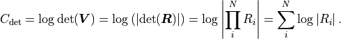
Numerical Considerations
The mathematical description of shown so far makes use of the inverse of the
covariance matrix  .
However, kafe2 does not actually calculate .
Instead the so-called QR decomposition
.
However, kafe2 does not actually calculate .
Instead the so-called QR decomposition  of the covariance matrix is being
used where
of the covariance matrix is being
used where  is an orthogonal matrix and
  is an upper triangular matrix.
Calculating
is an upper triangular matrix.
Calculating  is faster than calculating and it also reduces
the rounding error from floating point operations.
is faster than calculating and it also reduces
the rounding error from floating point operations.
Because is a triangular matrix
solving
the corresponding system of linear equations for the residual vector
 (difference between data and model) can be done very quickly:

With  and
and  we now find:

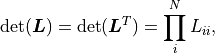
At the same time, because is an orthogonal matrix its determinant is either  or
or  .
is a triangular matrix and its determinant is simply the product of its diagonal values.
Valid covariance matrices have a positive determinant, so
.
is a triangular matrix and its determinant is simply the product of its diagonal values.
Valid covariance matrices have a positive determinant, so  can be efficiently calculated as:
Instead of a QR decomposition kafe2 can alternatively use a so-called Cholesky decomposition
with  where
where  is a lower triangular matrix.
The tradeoff is that a Cholesky decomposition is faster but less numerically stable than a QR decomposition.
Like with a QR decomposition the corresponding system of linear equations can be solved quickly:
is a lower triangular matrix.
The tradeoff is that a Cholesky decomposition is faster but less numerically stable than a QR decomposition.
Like with a QR decomposition the corresponding system of linear equations can be solved quickly:

and can be calculated as: